• Vehicular Networks

Vehicular Networks

---

Sample configuration files for all networks are available in Examples Menu in NetSim Home Screen. These files provide examples on how NetSim can be used – the parameters that can be changed and the typical effect it has on performance.

Importing a simple VANET scenario from SUMO #

Open NetSim and Select Examples > VANETs > Importing a simple VANET scenario from SUMO then click on the tile in the middle panel to load the example as shown in below screenshot.

Figure 4‑1: List of scenarios for the example of Importing a simple VANET scenario from SUMO

This scenario involves a simple road traffic network scenario as shown below:

Figure 4‑2: Network topology in Sumo

An equivalent network is created in NetSim by importing the SUMO configuration file. In NetSim the TCP/IP stack parameters of the devices are configured along with network traffic between vehicles.

Figure 4‑3: Network scenario after importing into NetSim and configuring application traffic

After running the simulation, NetSim Animation can be used to visualize packet flow and vehicle mobility along with packet information. Time varying throughput plot can be opened from the Results window.

Figure 4‑4: Packet animation window and link throughput plot

Simulation results dashboard provides the performance metrics of protocols running in different layers of the network stack of the devices.

Figure 4‑5: Result Dashboard

V2V and V2I communication involving Vehicles and RSUs #

Open NetSim and Select Examples > VANETs > V2V and V2I communication involving Vehicles and RSUs then click on the tile in the middle panel to load the example as shown in below screenshot

Figure 4‑6: List of scenarios for the example of V2V and V2I communication involving Vehicles and RSUs

NetSim VANETs module supports V2V and V2I communication. RSU's are now part of the GUI environment and can be dropped in addition to importing Vehicles from a SUMO configuration. Traffic can be configured between vehicles (V2V) and between vehicles and RSU’s (V2I).

This scenario involves a simple road traffic network scenario as shown below:

Figure 4‑7: Network topology in Sumo

An equivalent network is created in NetSim by importing the SUMO configuration file as shown below:

Figure 4‑8: Network set up for scenario involving vehicles and RSUs for v2v and v2i communication

After importing the SUMO configuration file in NetSim, RSU’s were added at junctions. In NetSim the TCP/IP stack parameters of the devices are configured along with network traffic between vehicles and between vehicles and RSU’s.

After running the simulation, NetSim Animation can be used to visualize packet flow and vehicle mobility along with packet information. Time varying throughput plot can be opened from the Results window.

Figure 4‑9: Packet animation window and link throughput plot

Simulation results dashboard provides the performance metrics of protocols running in different layers of the network stack of the devices.

Figure 4‑10: Result Dashboard

Throughput, delay and collisions with SCH and CCH time division #

All of the following examples are available in NetSim GUI. Navigate to Example > VANETs > Throughput, delay and collisions with SCH and CCH time division. Within Throughput, delay and collisions with SCH and CCH time division users will see four folders. Each folder comprises of simulation samples for Parts 1, 2, 3 and 4 as explained below.

Background#

Dedicated short range communication (DSRC) which uses two channels: Service channel SCH and Control channel (CCH). Each synchronization interval SI is split as follows

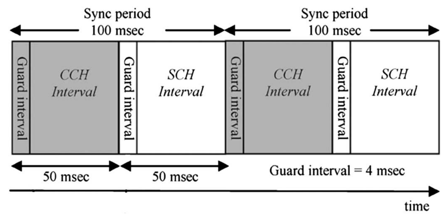
Figure 4‑11: We see the time divisions in DSRC. Each synchronization period consists of 1 CCH, 1 SCH and 1 guard interval. While the sync period is generally equal to 100 ms. NetSim allows users to modify the CCH and SCH interval, and in turn the total Sync period.

All devices switch between SCH and CCH and the alternation is based on the time divisions. NetSim allows the user to configure values of CCH interval, SCH interval and Guard interval. The default channels used in NetSim are SCH 171 (5.855 GHz) and CCH 178 (5.890 GHz)

Multiple nodes access the medium using 802.11p protocol. IEEE 802.11p PHY operates in the 5.9 GHz band with a channel bandwidth of 10 MHz 802.11p is an adaptation of the IEEE 802.11a standard used in Wi-Fi systems.

Simulation scenario#

Figure 4‑12: Illustration of the VANET scenario under study. The network comprises of 4 vehicles and 1 roadside unit. Each vehicle transmits two applications: (i) a BSM broadcast application that is sent to all other devices (vehicles plus RSU) within range and (ii) a CBR application transmitted to the RSU

The scenario comprises of four vehicles, V1, V2, V3 and V4 communication to the RSU, R1 and to one another. As explained in Figure 4‑11, each vehicle sends unicast CBR traffic to the RSU and broadcast BSM (safety messages) to one another. Recall that per DSRC functioning, BSM is sent on the CCH while CBR is sent on the SCH.

Simulation parameters and results#

Part 1: Throughput#

Open NetSim and Select Examples > VANETs > Throughput, delay and collisions with SCH and CCH time division > Throughput then click on the tile in the middle panel to load the example as shown in below screenshot

Figure 4‑13: List of scenarios for the example of Throughput

The following network diagram illustrates what the NetSim UI displays when you open the example configuration file throughput as shown in below Figure 4‑14.

Figure ‑: Network set up for studying the Throughput

Results#

The BSM application is configured with packet size of 20B and inter-packet arrival time of 320 μs, while the CBR application is configured with packet size of 1460B and inter-packet arrival time of 5840 μs.

Application	Application Type	Gen. Rate (Mbps)	CCH 20 ms SCH 80 ms	CCH 25 ms SCH 75 ms	CCH 30 ms SCH 70 ms	CCH 50 ms SCH 50 ms
			Throughput (Mbps)	Throughput (Mbps)	Throughput (Mbps)	Throughput (Mbps)
BSM 1	Broadcast	0.5	0.090	0.112	0.134	0.226
BSM 2	Broadcast	0.5	0.099	0.124	0.149	0.248
BSM 3	Broadcast	0.5	0.105	0.131	0.158	0.264
BSM 4	Broadcast	0.5	0.108	0.136	0.164	0.275
Sum Throughput (Mbps)			0.402	0. 504	0.605	1.014
Sum Throughput * (SCH+CCH)/CCH			2.011	2.015	2.017	2.027
CBR 1	Unicast	2	1.020	1.241	1.146	0.456
CBR 2	Unicast	2	0.695	0.667	0.903	0.868
CBR 3	Unicast	2	1.379	0.972	0.594	0.612
CBR 4	Unicast	2	1.808	1.626	1.553	1.109
Sum Throughput (Mbps)			4.902	4.507	4.195	3.045
Sum Throughput * (SCH+CCH)/SCH			6.127	6.009	5.993	6.090

Table 4‑1: We see that the as the CCH interval increases, BSM application has higher throughput rate. Similarly, as the SCH Interval decreases there is decrease in throughput rate.

Observations#

1. BSM in sent on CCH; CBR is sent on SCH. Increasing the fraction of time for CCH increases BSM throughput. Increasing the fraction of time for SCH increases CBR throughput.

2. As expected, Sum throughput divided by SCH fraction is equal for all cases. Similarly, Sum throughput divided by CCH fraction is equal in all cases. This verifies the working of time division between CCH and SCH.

Part 2: Delay#

Open NetSim and Select Examples > VANETs > Throughput, delay and collisions with SCH and CCH time division > Delay then click on the tile in the middle panel to load the example as shown in below screenshot

Figure 4‑15: List of scenarios for the example of Delay

The following network diagram illustrates what the NetSim UI displays when you open the example configuration file throughput as shown in below Figure 4‑16.

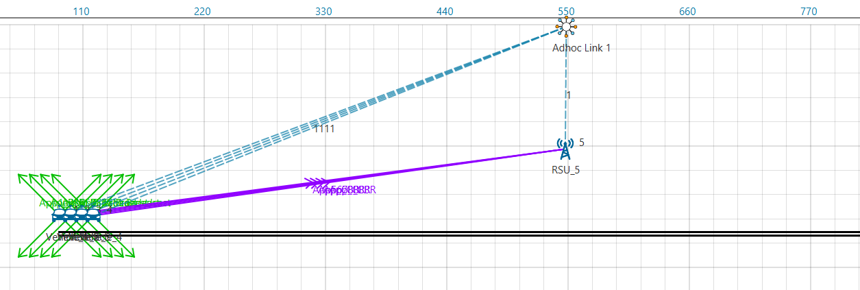
Figure ‑: Network set up for studying the Delay

Results#

When analyzing delay, we change the generation rate such that it is below the saturation capacity of the network. If this were not so, then queuing delay would blow-up at (and post) saturation.

Application	Application Type	Gen. Rate (Mbps)	CCH 20 ms SCH 80 ms	CCH 25 ms SCH 75 ms	CCH 30 ms SCH 70 ms	CCH 50 ms SCH 50 ms
			Delay (Micro sec)	Delay (Micro sec)	Delay (Micro sec)	Delay (Micro sec)
BSM 1	Broadcast	0.025	38774.178	33711.174	29184.264	15302.952
BSM 2	Broadcast	0.025	39085.500	33999.099	29580.397	15452.973
BSM 3	Broadcast	0.025	38871.482	34065.658	29612.045	15592.555
BSM 4	Broadcast	0.025	38971.652	34244.557	29722.204	15687.207
Average Delay			38925.703	34005.122	29524.728	15508.922
CBR 1	Unicast	1	970820.956	623360.782	1070605.026	3231622.594
CBR 2	Unicast	1	554478.563	1711244.232	938543.697	3167638.761
CBR 3	Unicast	1	660493.934	1021442.963	1682596.057	3767856.679
CBR 4	Unicast	1	827215.500	694044.413	1435345.051	4040215.389
Average Delay			753252.238	1012523.097	1281772.458	3551833.356

Table 4‑2: We see that as the CCH interval increases, the delay for BSM application decreases. Similarly, as the SCH interval decreases the delay for CBR application increases.

Observations#

1. CCH Delay has 3 components (a) waiting time where the packet is waiting for the SCH to complete (b) Medium access time and (c) Transmission time

2. The mathematical analysis of delay is complex. It involves two evaluating two difficult components (i) CCH packet waiting time while SCH packet is served and vice versa, and (ii) medium access time. We leave the mathematical analysis to interested researchers, and restrict ourselves to stating that the trends are as expected i.e., increasing CCH time (and reducing SCH time) reduces the CCH delay (and increases SCH delay)

Part 3: Collision count with increasing generation rate#

Open NetSim and Select Examples > VANETs > Throughput, delay and collisions with SCH and CCH time division > Collision count with increasing generation rate then click on the tile in the middle panel to load the example as shown in below screenshot

Figure 4‑17: List of scenarios for the example of Collision count with increasing generation rate

The following network diagram illustrates what the NetSim UI displays when you open the example configuration file throughput as shown in below Figure 4‑18.

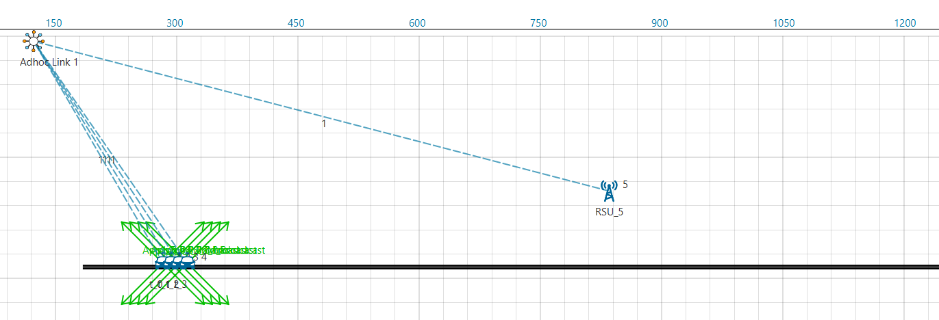
Figure ‑: Network set up for studying the Collision count with increasing generation rate

Figure ‑: The scenario layout remains the same, however we change the application settings. In this example we only have the 4 BSM applications. There are no CBR applications.

Results#

The application generation rates are mentioned in Row 1 (shaded grey).

Application	Application Type	Gen Rate 0.005 Mbps	Gen Rate 0.010 Mbps	Gen Rate 0.015 Mbps	Gen Rate 0.020 Mbps
		Collision Count	Collision Count	Collision Count	Collision Count
BSM 1	Broadcast	1148	2686	4347	6157
BSM 2	Broadcast	826	1897	3049	4337
BSM 3	Broadcast	617	1298	2223	3014
BSM 4	Broadcast	474	1034	1670	2370
Total collisions		3065	6915	11289	15878
Total pkts transmitted		28934	57818	86720	115578
Collision Probability		0.106	0.120	0.130	0.137

Table 4‑3: Comparison of Collision count of BSM applications with changing generation rate

The Collision probability is the ratio between Collision count to total number of packets transmitted

$$Collision\ probability = \ \frac{Collision\ count}{packets\ transmitted}$$

To find the Collision count of each individual application,

• Click on Packet Trace in the results dashboard window (Please make sure the packet trace is enabled before running the simulation)

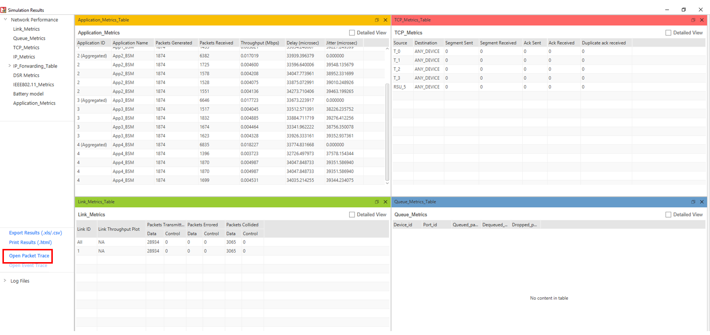
Figure ‑ : Results dashboard window

• total no of collision counts and packets transmitted can be viewed in the link metrics table over results dashboard

• In packet trace, filter the control packet type/ App Name to App1_BSM to find the individual collision count

• Along with that filter the packet status field to collisions to view the collisions of that particular application (APP1_BSM)

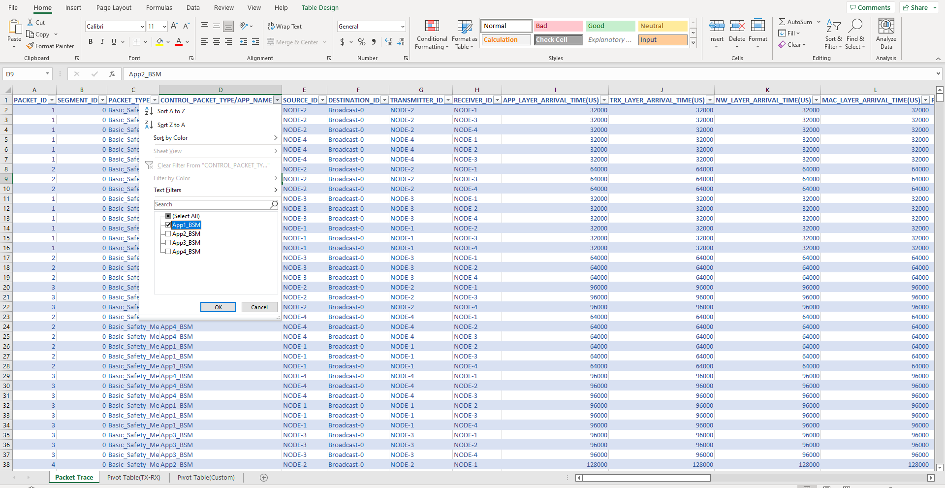
Figure ‑ : Packet trace which depicts filtering of applications

Figure ‑ : Packet trace that depicts filtering of packet status of each application

• After applying the filters, the total collision count of APP1_BSM applications can be viewed

Figure ‑ : packet trace

• Same process can be done for all the remaining applications of the network.

Observations#

• Saturation throughput is about 0.25 Mbps per app or 1 Mbps total. Note the generation rate is below the saturation capacity of the network

• We see collision probability increases as generation rate increases

• To the best of our knowledge the mathematical modelling of collisions with non-saturated queues is an open problem. The Bianchi model exists for predicting collision counts with saturated queues, subject to certain conditions.

Part 4: Collisions count with increasing number of nodes#

Open NetSim and Select Examples > VANETs > Throughput, delay and collisions with SCH and CCH time division > Collisions count with increasing number of nodes then click on the tile in the middle panel to load the example as shown in below screenshot

Figure 4‑24: List of scenarios for the example of Collisions count with increasing number of nodes

The following network diagram illustrates what the NetSim UI displays when you open the example configuration file throughput as shown in below Figure 4‑21 [1]

Figure ‑: Network set up for studying the Collisions count with increasing number of nodes

This scenario has 10 vehicles in a line on a road. The vehicles transmit power P_t = 20 dBm, Carrier sense threshold CS_th=  − 85 dBm, and we assumed log distance pathloss with η = 2.5. The received power between nodes with maximum separation, d = 100, is

P_r = 20 − 47.88 − 10 × 2.5 × log (100)=  − 77.88 dBm

Since P_r > CS_th all nodes can hear one another which means that they are all within CS Range.

Figure ‑: Illustration of the VANET scenario under study. The network comprises of 10 vehicles and 1 roadside unit. Each vehicle transmits one application (i) a BSM broadcast application that is sent to all other devices (vehicles plus RSU) within range. In this study we are increasing the Tx nodes from 1-10

Results#

Number of Tx nodes	Collision Count	Pkts transmitted	Collision Probability
1	0	24786	0.000
2	5297	69515	0.076
3	15080	127398	0.118
4	28723	179751	0.160
5	45665	244391	0.187
6	66506	316725	0.210
7	89357	396539	0.225
8	127606	490200	0.260
9	166575	586842	0.284
10	216332	694672	0.311

Table 4‑4: Collision probability comparison with change in number of transmitting nodes

The total no of collision count and packets transmitted can be viewed in link metrics window of results dashboard

Figure 4‑27 : Results Dashboard window

The Collision probability is the ratio between Collision count to total number of packets transmitted

$$Collision\ probability = \ \frac{Collision\ count}{packets\ transmitted}$$

Figure 4‑28: Collision probability vs. number of transmitting nodes

Observations#

• We see collision count increasing with number of transmitting nodes

• This can be compared against the Bianchi analytical model

SUMO Manhattan Mobility with Single and Multi-hop Communication #

Introduction

The Manhattan mobility in SUMO features a grid topology as shown below. It is composed of a number of horizontal and vertical streets. Each street has two lanes for each direction (North and South direction for vertical streets, East and West for horizontal streets). The mobile node is allowed to move along the grid of horizontal and vertical streets. At an intersection of a horizontal and a vertical street, the mobile node can turn left, right or go straight with certain probability.

Figure 4‑29: Manhattan mobility in SUMO features a grid topology

Case 1: Manhattan mobility Single-hop RSU to vehicles

Objective

To create, using SUMO, a Manhattan Road network in which vehicles drive randomly, and to have a Roadside unit (RSU) which sends safety messages continuously to vehicles. The network performance is analyzed for different environments each having different RF channel characteristics.

Procedure

Open NetSim and Select Examples > VANETs > SUMO Manhattan mobility > Single hop communication then click on the tile in the middle panel to load the example as shown in below screenshot

Figure 4‑30: List of scenarios for the example of Single hop communication

The NetSim UI would display as shown below.

Figure 4‑31: Network set up for studying the Single hop communication

Settings done for this sample experiment.

1. Applications set as CBR (Broadcast application)

Application Method	Application Type	Application Name	Source ID	Destination ID		Packet Size (Bytes)	Inter-Arrival Time (µs)
Broadcast	CBR	APP_1_CBR_ Broadcast	21	Broadcast to all 20 vehicles	300		2,000,000

Table 4‑5: CBR Applications Settings

1. Transport protocol set as UDP in application Configuring window.

2. Adhoc link/Wireless link properties were set as follows:

Channel characteristics	Pathloss Model	Pathloss Exponent
Pathloss Only	Log Distance	2.5

Table 4‑6: Wireless link properties

1. Co-ordinates of RSU are set as X = 834.62, and Y = 133.85.

2. Set transmitter power to 40mW under INTERFACE_1(Wireless) > Physical layer properties of Vehicles and RSU.

3. Plots and packet trace are enabled and run simulation and observe the movement of the vehicles in the packet animation window.

4. In NetSim packet animation window, you can see that vehicles choose random directions when they reach a junction in the Manhattan grid network.

5. Increase the pathloss exponent (in the order 2.5, 3, 3.5, 4) and note down the aggregate throughput and packets received for different application generation rates.

Figure 4‑32: Animation Window for NetSim

With play and record animation enabled, same can be observed in SUMO as follows:

Figure 4‑33: Animation Window for Sumo

Results and Observations

For sample RSU Broadcast Data Rate = 1.2 Kbps (Packet size = 300 bytes, IAT = 2,000,000µs. This means packets of size 300 Bytes are sent every 2 seconds).

Environment	Path-loss Exponent	Packets Received (Aggregate)*	Throughput (Kbps) (Aggregate)
Open Rural Area	2.5	198	4.752
Urban Area	3	59	1.41
Dense Urban Area	3.5	14	0.33
Very Dense Urban Area with Shadowing	4	2	0.048

Table 4‑7: Results Comparison for RSU Broadcast Data Rate = 1.2 Kbps

* Aggregate is the sum of the packet/throughputs obtained by all applications.

For sample RSU Broadcast Data Rate = 2.4 Kbps (Packet size =300 Bytes, IAT = 1,000,000µs or 1 seconds. This means packets of size 300 Bytes are sent every second)

Environment	Path-loss Exponent	Packets Received (Aggregate)	Throughput (Kbps) (Aggregate)
Open Rural Area	2.5	397	9.528
Urban Area	3	119	2.856
Dense Urban Area	3.5	26	0.624
Very Dense Urban Area with Shadowing	4	4	0.096

Table 4‑8: Results Comparison for RSU Broadcast Data Rate = 2.4 Kbps

For sample RSU Broadcast Data Rate = 9.6 Kbps (Packet size =300Bytes, IAT =250,000µs or 0.25 seconds. This means four packets of size 300 Bytes are sent every second)

Environment	Path-loss Exponent	Packets Received (Aggregate)	Throughput (Kbps) (Aggregate)
Open Rural Area	2.5	1593	38.232
Urban Area	3	482	11.56
Dense Urban Area	3.5	102	2.448
Very Dense Urban Area with Shadowing	4	16	0.384

Table 4‑9: Results Comparison for RSU Broadcast Data Rate = 9.6 Kbps

Figure 4‑34: Plot of Throughput vs. Pathloss Exponent for different RSU broadcast for different DR (Data Rates)

Case 2: Manhattan mobility Multi-hop Vehicles to RSU

Objective

To create, using SUMO, a Manhattan Road network in which vehicles drive randomly, and to have a Roadside unit (RSU) to which vehicles continuously send unicast traffic via multi-hop (hopping via other vehicles if the RSU is beyond communication range). The network performance is analyzed for different vehicle counts.

Procedure

Open NetSim and Select Examples > VANETs > SUMO Manhattan mobility > Multi hop communication then click on the tile in the middle panel to load the example

Figure 4‑35: List of scenarios for the example of Multi hop communication

The NetSim UI would display as shown below.

Figure 4‑36: Network set up for studying the Multi hop communication

Settings done for this sample experiment.

1. Applications set as CBR.

Application Method	Application Type	Source_Id	Destination_Id	Packet size (Bytes)	Inter-Arrival Time (µs)
Unicast	CBR	(All vehicles)	RSU	1460	20,000

Table 4‑10: CBR Applications settings

1. In Vehicle General Properties, under SUMO file manhattan.sumo.cfg file was selected from the Docs folder of NetSim Install Directory \< C:\Program Files\NetSim Standard\Docs\Sample_Configuration\VANET\SUMO-Manhattan-mobility-Single-hop-and-Multi-hop\Multi-hop-communication>

Figure 4‑37: General Properties window

1. Transport protocol set as UDP in application Configuration window.

2. Adhoc link/ Wireless link properties set as follows:

Channel Characteristics Pathloss Model Pathloss Exponent Pathloss Only Log Distance 2.5

Figure 4‑38: Wireless link properties

1. Co-ordinates of RSU are set as X = 450, and Y = 450

2. Network layer routing protocol is set as DSR.

3. Set transmitter power to 40mW under INTERFACE_1(Wireless) > Physical layer properties of Vehicles and RSU.

4. Plots are enabled and run the simulation.

5. Increase the number of vehicles in the order 10, 20, 30 etc. and note down the aggregate throughput.

Result:

Number of vehicles	Throughput (Kbps) (Aggregate)*
10	1.1826
20	0.5405
30	0.6668
40	1.1857
50	1.0780
60	0.9119
70	0.5720

Table 4‑11: Results Comparison

*Aggregate is the sum of the packet/throughputs obtained by all applications.

Figure 4‑39: Aggregate Throughput vs. Number of Vehicles

SUMO Interfacing with vehicles moving in a closed loop #

Open NetSim and Select Examples > VANETs > SUMO Vehicles in closed loop then click on the tile in the middle panel to load the example as shown in below screenshot

Figure 4‑40: List of scenarios for the example of SUMO Vehicles in closed loop

The NetSim UI would display as shown below.

Figure 4‑41: Network set up for studying the SUMO Vehicles in closed loop

Settings done for this sample experiment:

1. Applications set as BSM (Basic_Safety_Message)

APP_ID	Source ID	Destination ID	Packet Size (Bytes)	Inter-Arrival Time (µs)
APP_1_BSM	1	6 (RSU)	100	2,000,000
APP_2_BSM	2	6 (RSU)	100	2,000,000
APP_3_BSM	3	6 (RSU)	100	2,000,000

Table 4‑12: CBR Applications settings

1. Transport protocol set as WSMP for all applications in Application window.

2. In Vehicle General Properties, under SUMO file Configuration.sumo.cfg file was selected from the Docs folder of NetSim Install Directory \< C:\Program Files\NetSim Standard\Docs\Sample_Configuration\VANET\SUMO-Vehicles-moving-in-closed-loop >

Figure 4‑42: General Properties window

1. Adhock link/Wireless link properties were set as follows:

Channel Characteristics	Pathloss Model	Pathloss Exponent
Pathloss_Only	Log_Distance	2

Table 4‑13: Wireless link properties

1. Co-ordinates of RSU are set as X = 278.31 and Y = 153.48

2. Medium access protocol set as DCF in all vehicles and RSU.

3. Set transmitter power to 40mW under INTERFACE_1(Wireless) > Physical layer properties of Vehicles and RSU.

4. Enable Plot and Run simulation and observe the movement of the vehicles in the packet animation window.

5. After the simulation, in NetSim Packet Animation window, we can see that vehicles are moving continuously through the closed-loop hexagonal path till the given end time.

Result:

Figure 4‑43: Packet animation window for NetSim

With play and record animation enabled, same can be observed in SUMO as well

Figure 4‑44: Animation window for Sumo

According to SUMO, the road network consist of ‘Edges’ and ‘Junctions’. The re-router (a device in SUMO and is not to be confused with Routers available in NetSim) established in the edge will re-route the vehicle from one edge to other after one successful revolution through the road network. The presence of a single re-router will forward the vehicles from one edge to other and then the vehicle eventually stops its movement. Hence, two re-routers have been established in two edges which re-routes the vehicle from one edge to other. The above road network consists of six edges in which re-routers are established in the starting and ending edges, which re-routes the vehicles present in the network from starting edge to the finishing edge after one complete revolution through the road or path. As a result, the vehicles will move through the closed loop continuously, until the end time configured in the configuration file.

In the animation window, we can observe that the vehicles will start from a point in one of the edges, moves through other five edges and finally reach back the point where it started. At this point, the re-router will direct the vehicles to the next edge. This cycle will continue till the end time configured.

The RSU configured in the network will allow V2I communication. Per the application configuration a 100 bytes packet is transmitted from vehicle to RSU every 2 seconds. This can also be observed in the packet trace.