• 5G-NR

5G-NR

---

Understand 5G simulation flow through LTENR log file#

Open NetSim, Select Examples ->5G NR ->5G Log File and Packet Trace then click on the tile in the middle panel to load the example as shown in below screenshot

Figure 4‑1: List of scenarios for the example: 5G Log File and Packet Trace

The following network diagram illustrates, what the NetSim UI displays when you open the example configuration file.

Figure 4‑2: Network set up for studying the 5G Log File and Packet Trace

Settings done in example config file:

1. CBR application source id as 10 and destination id as 8 with Packet_Size as 1460 and InterArrival_Time as 20000 (Generation rate of 0.584 Mbps). Transport Protocol is set to UDP.

2. Set other properties to default.

3. The log file can enable per the information provided in Section 3.18.

4. Enable Plots, Packet Trace and Run Simulation for 10s.

To view and study the 5GNR design/flow of the simulation, use the LTENR.log file which can be opened post simulation from Results Window > Log Files.

For logging additional information relating to Buffer-status-notification, open the source code and inside the LTE NR project, uncomment the lines given below in LTE_NR.h

LTE_NR.h

#define LTENR_LOG_DEV

#define LTENR_PDCP_LOG

#define LTENR_RLC_BUFFERSTATUSREPORTING_LOG

• *

Figure 4‑3: LTENR code uncomment to log Buffer-status-notification and Transmission-status-notification

Rebuild the code to enable logs per Section 3.18 in the 5G-NR manual. Note that log files would generally be quite large (>10 MB of size). In the GUI enable packet trace and event trace before running the simulation. Run the simulation. Open the packet trace and ltenr.log file from the results window.

1. The Physical Resource Block (PRB) list is formed at the beginning of the log file. This corresponds to 1 slot $\left( \frac{1}{2^{\mu}}\ ms \right)$ in time-domain and 15 * 12 * 2^μ kHz in frequency domain.

Figure 4‑4: LTE NR Log File: PRB List

1. The naming convention used in the ltenr log file is gNB \<gnb ID>:\<Interface>. For example, gNB 7:4 means gNB 7 interface 4.

2. For each numerology and carrier, a resource grid of (max. number of > resource blocks for that numerology) * (number of sub-carriers > per resource block) and (number of symbols per sub-frame of that > numerology) is defined.

3. In this example the GUI settings (gNB 5G-RAN interface Physical > Layer) are:

   • μ (numerology) is set 0.

   • No. of resource blocks (PRB count) = 52

   • No. of sub-carriers per PRB = 12

   • No. of symbols per sub-frame of numerology (0) = 1.

4. The log file explains the PRB list for gNB (7) on interface (4):

   • The lowest (F_Low_MHz) and highest frequency (F_High_MHz) for > the Uplink/Downlink operating bands are logged first along > with the channel bandwidth (MHz), PRB bandwidth(kHz) and guard > bandwidth(kHz).

   • The list defines the lower frequency, upper frequency, and > central frequency in MHz for each physical resource block of > the PRB count.

Figure 4‑5: LTE NR Log File: Lower, Higher and Central Frequencies for PRB List

1. The UE association/dissociation is done which is logged. UE (8) on interface (1) associates with gNB (7) on interface (4). During UE association:

2. The Adaptive Modulation and Coding (AMC) information is initialized > for Uplink and Downlink:

   • AMC information: Links Spectral efficiency is calculated and > based on this Channel quality indicator (CQI) (Includes the > CQI index, modulation, code rate and efficiency) and > Modulation coding scheme (MCS) (Includes the MCS index, > modulation, modulation order, code rate and spectral > efficiency) is read from the standard table and setup for both > Downlink and Uplink.

Figure 4‑6: LTE NR Log File: UE Association

1. The numerology is equal to 0, hence the slots/sub-frame = 1 and there will be 10 sub-frames per frame. Accordingly, the frames, sub-frames and slots are created as shown below:

2. A new frame gets started for the gNB, where the frame id=1, start > time and the end time of the frame are logged.

3. After the frame-1 starts, the sub-frame for the same gnb is started > within the frame. The frame id=1, sub-frame id=1, start time and > end time are logged

4. Within frame-1, sub-frame-1 a slot is started. This slot’s ID (1), > slot type (Uplink), start time and end time are logged.

Figure 4‑7: LTE NR Log File: Frame and Sub Frame list with start time and end time

1. The RLC-sublayer will check the UE buffer for packets. Based on the logical channel (DTCH) and the transmission mode (UM, AM), the entity is identified, and the buffer size of each mode is read. The combined buffer size of all the modes gives the total buffer size (number of bytes to be processed).

2. The RLC sub-layer then processes the transmission status notification for downlink:

3. Initially the RLC transmission for the control takes place, where > the transmission status for each of the control logical channels > i.e., BCCH, CCCH, DCCH and PCCH is calculated based on the mode > (TM & AM) they support.

4. While calculating the transmission status for control, the RLC sends > the Physical Data Unit (PDU) based on the mode (TM or AM).

5. Later the RLC transmission for the data packet happens, where the > transmission status for traffic logical channel i.e., DTCH is > calculated based on the AM and UM mode it supports.

6. DTCH channel supports Un-Ack mode (UM). It checks for the buffer and > if the buffer isn’t NULL:

   • It will find the buffer that matches the logical channel, and it > only proceeds further if the size of the PDU is within the > minimum RLC PDU size.

   • If the message packet is NULL (or) message type is user data & > the payload of PDU is greater than size of PDU, it fragments > the UM data buffer packet (or else) the buffer is marked for > removal.

   • Then the RLC sends the PDU to the MAC layer. And then the RLC > buffer gets updated.

7. At time 1000502.4 µs packet arrives at the Service Data Adaptation Protocol (SDAP) sub layer in the gNB:

8. As the packet arrives at the SDAP sub-layer, the SDAP header is > appended to the Packet with header size.

9. SDAP sets the RLC mode (here, acknowledge mode) based on QoS, and > the logical channel (DTCH) is chosen.

10. The packet is passed to the Packet Data Convergence Protocol (PDCP) sub-layer at gNB:

11. Packet is enqueued to the transmission (Tx) buffer and discard time > is started.

12. PDCP header is added, and packet is passed to the RLC sub-layer.

13. The packet is then passed to the Radio Link Control (RLC) sub-layer at gNB and is added to the transmission buffer.

Figure 4‑8: LTE NR Log File: SDAP, PDCP and RLC sublayers

1. Now a new sub frame id - 2 with slot id - 1 gets created for the frame id - 1. Here the slot type (Downlink)

Figure 4‑9: LTE NR Log File: Frame Id and slot Id

1. The RRC related packets like RRC_MIB, RRC_SIB1 arrives are RLC Sub-layer and the packets are added to the transmission buffer.

Figure 4‑10: LTE NR Log File: RRC Packet details

1. The data packet is sent from the transmission buffer in DTCH logical channel (for downlink) from gNB to UE. This packet is sent to the MAC sub-layer and the packet is then added to the transmitted buffer.

2. The packet enters the Radio Link Control (RLC) protocol sub-layer in the MAC layer at the UE:

3. The PDU (Physical Data Unit) is received at the UE, specific to RLC > mode:

4. The AMPDU header of the packet is received and logged. If the > sequence number of the PDU is outside the receiving window, the > PDU is discarded.

5. It checks if the PDU is already present in the reception buffer. If > present it drops the PDU and if the PDU is not present in the > reception buffer, then it is added to the reception buffer: The > sequence index (SI), sequence number (SN), and sequence order (SO) > for the corresponding mode also get updated.

6. Checks if all the Service Data Unit (SDU) byte segments of the PDU > packet have been received. If not, it waits for the remaining > SDU’s before transmitting packet. The reassembly is done for all > the SDU if all the SDU byte segments of PDU packet are received.

7. Checks if the reassembly timer is started or not and stops if > started and vice-versa.

8. And the status report of RLC-AM is set as delayed.

Figure 4‑11: LTE NR Log File: MAC sublayer, AMDPDU Header

1. If the header exists, the STATUSPDU is constructed, else the status will be marked as delayed and the packet will pass to TM mode for transmission. PDU is handed over to RLC TM mode and packet gets added to transmission buffer.

Figure 4‑12: LTE NR Log File: STATUSPDU Construction

1. The packet is received by the PDCP sub-layer. The PDCP state variables like the receive sequence number(sn), receive hyper frame number(hfn) and the receive count are calculated.

2. Next the STATUSPDU gets transmitted from the UE to the gNB (See Packet Trace)

Figure 4‑13: 5G NR Packet Trace

1. The packet enters the Radio Link Control (RLC) protocol sub-layer in the MAC layer at the UE. Specific to the RLC mode (TM), it receives the Physical Data Unit (PDU) at the UE:

2. Based on the control data type of the packet, the case is chosen.

3. Since it is STATUSPDU type, the STATUSPDU packet is received > accordingly at the gNB. And the RLCAM transmitted buffer is > cleared, and poll retransmit timer is stopped.

Effect of distance on pathloss for different channel models #

Open NetSim, Select Examples ->5G NR ->Distance vs Pathloss then click on the tile in the middle panel to load the example as shown in below screenshot

Figure 4‑14: List of scenarios for the example of Distance vs Pathloss

The following network diagram illustrates, what the NetSim UI displays when you open the example configuration file.

Figure 4‑15: Network set up for studying the Distance vs Pathloss

Rural-Macro#

Line-of-Sight (LOS)#

Settings done in example config file

1. Set distance between gNB_7 and UE_8 as 30m.

2. Go to gNB properties à Interface (5G_RAN) à PHYSICAL_LAYER.

Properties
CA Type	INTER_BAND_CA
CA Configuration	CA_2DL_1UL_n39_n41
Pathloss Model	3GPPTR38.901-7.4.1
Outdoor_Scenario	RURAL_MACRO
LOS_NLOS_Selection	USER_DEFINED
LOS_Probabillity	1
Shadow Fading Model	None
Fading_and_Beamforming	NO_FADING_MIMO_UNIT_GAIN
O2I Building Penetration Model	None

Table 4‑1: gNB >Interface (5G_RAN) >Physical layer properties

Note: HARQ mode in gNB properties à Interface (5G_RAN) à Datalink layer is disabled in all 5G featured examples.

1. CBR application source id as 10 and destination id as 8 with packet size as 1460Bytes and Inter_Arrival_time as 20000μs (Generation Rate=0.584). Transport Protocol is set to UDP. Additionally, the “Start Time(s)” parameter is set to 1s, while configuring the application.

2. Set UE height as 10m.

3. Set other properties to default.

4. Plots are enabled in NetSim GUI.

5. The LTENR Radio measurement log file must be enabled as per information provided in the section 3.19.

6. Run Simulation for 20s, after the simulation completes Go to metrics window expand Log Files option and open LTENR Radio Measurement Log.csv and note down the Pathloss.

Figure 4‑16: Results window

Figure 4‑17: LTENR Radio Measurement log.csv file

Go back to the scenario and change the distance between gNB and UE as 30, 50, 70, 100, 300, 500, 700, and 1000 and note down Pathloss value from the log file.

Non-Line-of-Sight (NLOS)#

Settings done in example config file

1. Set distance between gNB_7 and UE_8 as 30m.

2. Go to gNB properties à Interface (5G_RAN) à PHYSICAL_LAYER.

Properties
CA Type	INTER_BAND_CA
CA Configuration	CA_2DL_1UL_n39_n41
Pathloss Model	3GPPTR38.901-7.4.1
Outdoor_Scenario	RURAL_MACRO
LOS_NLOS_Selection	USER_DEFINED
LOS_Probabillity	0
Shadow Fading Model	None
Fading _and_Beamforming	NO_FADING_MIMO_UNIT_GAIN
O2I Building Penetration Model	None

Table 4‑2: gNB >Interface (5G_RAN) >Physical layer properties

1. Set all other properties same as LOS example.

2. Plots are enabled in NetSim GUI.

3. The LTENR Radio measurement log file can be enabled as per information provided in the section 3.19.

4. Run Simulation for 20s.

Go back to the scenario and change the distance between gNB and UE as 30, 50, 70, 100, 300, 500, 700, and 1000 and note down Pathloss value from the log file.

Result#

Distance(m)	LOS Pathloss(dB)			NLOS pathloss (dB)
	CA 1	CA 2	Avg	CA 1	CA 2	Avg
30	67.60	70.30	68.95	69.03	71.73	70.38
50	72.17	74.87	73.52	77.97	80.67	79.32
70	75.19	77.89	76.54	83.86	86.56	85.21
100	78.41	81.11	79.76	90.11	92.81	91.46
300	88.46	91.16	89.81	109.35	112.05	110.70
500	93.28	95.98	94.63	118.29	120.99	119.64
700	96.55	99.25	97.90	124.18	126.88	125.53
1000	100.14	102.84	101.49	130.43	133.13	131.78

Table 4‑3: Results Comparison for LOS and NLOS pathloss vs. Distance

Figure 4‑18: Plot of Distance vs. Avg Pathloss

Urban-Macro#

Line-of-Sight (LOS)#

Settings done in example config file

1. Set distance between gNB_7 and UE_8 as 30m.

2. Go to gNB properties à Interface (5G_RAN) à PHYSICAL_LAYER

Properties
CA Type	INTER_BAND_CA
CA Configuration	CA_2DL_1UL_n39_n41
Pathloss Model	3GPPTR38.901-7.4.1
Outdoor_Scenario	URBAN_MACRO
LOS_NLOS_Selection	USER_DEFINED
LOS_Probabillity	1
Shadow Fading Model	None
Fading_and_Beamforming	NO_FADING_MIMO_UNIT_GAIN
O2I Building Penetration Model	None

Table 4‑4: gNB >Interface (5G_RAN) >Physical layer properties

1. CBR application source id as 10 and destination id as 8 with packet size as 1460Bytes and Inter_Arrival_time as 20000μs (Generation Rate=0.584). Transport Protocol is set to UDP. Additionally, the “Start Time(s)” parameter is set to 1s, while configuring the application.

2. Set UE height as 10m.

3. Set other properties to default.

4. Plots are enabled in NetSim GUI.

5. The LTENR Radio measurement log file can be enabled as per information provided in the section 3.19

6. Run Simulation for 20s, after the simulation completes Go to metrics window expand Log Files option and open LTENR Radio Measurement Log.csv and note down the pathloss.

Figure 4‑19: Result window

Figure 4‑20: LTENR Radio Measurement log.csv file

Go back to the scenario and change the distance between gNB and UE as 30, 50, 70, 100, 300, 500, 700, and 1000 and note down Pathloss value from the log file.

Note: The minimum distance for rural macro and urban macro is 35m. Below 35m, the 2D and 3D distance will be 10m in ltenr log file.

Non-Line-of-Sight (NLOS)#

Settings done in example config file

1. Set distance between gNB_7 and UE_8 as 30m.

2. Go to gNB properties à Interface (5G_RAN) à PHYSICAL_LAYER

Properties
CA Type	INTER_BAND_CA
CA Configuration	CA_2DL_1UL_n39_n41
Pathloss Model	3GPPTR38.901-7.4.1
Outdoor_Scenario	URBAN_MACRO
LOS_NLOS_Selection	USER_DEFINED
LOS_Probabillity	0
Shadow Fading Model	None
Fading_and_Beamforming	NO_FADING_MIMO_UNIT_GAIN
O2I Building Penetration Model	None

Table 4‑5: gNB >Interface (5G_RAN) >Physical layer properties

1. Set all other properties same as LOS example.

2. Plots are enabled in NetSim GUI.

3. The log file can enable per the information provided in Section 3.18

1. Run Simulation for 20s, after the simulation completes Go to metrics window expand Log Files option and open LTENR Radio Measurement Log.csv and note down the pathloss.

1. Go back to the scenario and change the distance between gNB and UE as 30, 50, 70, 100, 300, 500, 700, and 1000 and note down Pathloss value from the log file.

Result#

Distance(m)	LOS Pathloss(dB)			NLOS pathloss (dB)
	CA 1	CA 2	Avg	CA 1	CA 2	Avg
30	66.07	68.77	67.42	71.74	74.44	73.09
50	70.95	73.65	72.30	80.41	83.11	81.76
70	74.16	76.86	75.51	86.12	88.82	87.47
100	77.57	80.27	78.92	92.17	94.87	93.52
300	88.07	90.77	89.42	110.82	113.52	112.17
500	92.95	95.65	94.30	119.49	122.19	120.84
700	96.16	98.86	97.51	125.20	127.90	126.55
1000	99.57	102.27	100.92	131.25	133.95	132.60

Table 4‑6: Results Comparison for LOS and NLOS pathloss vs. Distance

Figure 4‑21: Plot of Distance vs. Avg Pathloss

Urban-Micro#

Line-of-Sight (LOS)#

Settings done in example config file

1. Set distance between gNB_7 and UE_8 as 30m.

2. Go to gNB properties à Interface (5G_RAN) à PHYSICAL_LAYER

Properties
CA Type	INTER_BAND_CA
CA Configuration	CA_2DL_1UL_n39_n41
Pathloss Model	3GPPTR38.901-7.4.1
Outdoor_Scenario	URBAN_MICRO
LOS_NLOS_Selection	USER_DEFINED
LOS_Probabillity	1
Shadow Fading Model	None
Fading _and_Beamforming	NO_FADING_MIMO_UNIT_GAIN
O2I Building Penetration Model	None

Table 4‑7: gNB >Interface (5G_RAN) >Physical layer properties

1. CBR application source id as 10 and destination id as 8 with packet size as 1460Bytes and Inter_Arrival_time as 20000μs (Generation Rate=0.584). Transport Protocol is set to UDP. Additionally, the “Start Time(s)” parameter is set to 1s, while configuring the application.

2. Set UE height as 10m.

3. Set other properties to default.

4. Plots are enabled in NetSim GUI.

5. The LTENR Radio measurement log file can be enabled as per information provided in the section 3.19

6. Run Simulation for 20s, after the simulation completes Go to metrics window expand Log Files option and open LTENR Radio Measurement Log.csv and note down the Pathloss.

Figure 4‑22: Result window

Figure 4‑23: LTENR Radio Measurement log.csv file

Go back to the scenario and change the distance between gNB and UE as 30, 50, 70, 100, 300, 500, 700, and 1000 and note down Pathloss value from the log file.

Non-Line-of-Sight (NLOS)#

Settings done in example config file

1. Set distance between gNB_7 and UE_8 as 30m.

2. Go to gNB properties à Interface (5G_RAN) à PHYSICAL_LAYER.

Properties
CA Type	INTER_BAND_CA
CA Configuration	CA_2DL_1UL_n39_n41
Pathloss Model	3GPPTR38.901-7.4.1
Outdoor_Scenario	URBAN_MICRO
LOS_NLOS_Selection	USER_DEFINED
LOS_Probabillity	0
Shadow Fading Model	None
Fading_and_Beamforming	NO_FADING_MIMO_UNIT_GAIN
O2I Building Penetration Model	None

Table 4‑8: gNB >Interface (5G_RAN) >Physical layer properties

1. Set all other properties same as LOS example.

2. Plots are enabled in NetSim GUI.

3. The log file can enable per the information provided in Section 3.18.

4. Run Simulation for 20s, after the simulation completes Go to metrics window expand Log Files option and open LTENR Radio Measurement Log.csv and note down the pathloss.

5. Go back to the scenario and change the distance between gNB and UE as 30, 50, 70, 100, 300, 500, 700, and 1000 and note down Pathloss value from the log file.

Result#

Distance(m)	LOS Pathloss (dB)			NLOS pathloss (dB)
	CA 1	CA 2	Avg	CA 1	CA 2	Avg
30	68.99	71.69	70.34	77.92	80.80	79.36
50	73.65	76.35	75.00	85.76	88.63	87.195
70	76.72	79.42	78.07	90.91	93.79	92.35
100	79.97	82.67	81.32	96.38	99.26	97.82
300	89.99	92.69	91.34	113.22	116.10	114.66
500	94.65	97.35	96.00	121.06	123.93	122.495
700	97.72	100.42	99.07	126.21	129.09	127.65
1000	100.97	103.67	102.32	131.68	134.56	133.12

Table 4‑9: Results Comparison for LOS and NLOS pathloss vs. Distance

Figure 4‑24: Plot of Distance vs. Avg Pathloss

Indoor-Office#

The following network diagram illustrates, what the NetSim UI displays when you open the example configuration file.

Figure 4‑25: Network Topology for this experiment

Line-of-Sight (LOS)#

Settings done in example config file

1. Drop the building and drop gNB and UE inside the building.

2. Set distance between gNB_7 and UE_8 as 10m.

3. Go to gNB properties à Interface (5G_RAN) à PHYSICAL_LAYER.

Properties
CA Type	INTER_BAND_CA
CA Configuration	CA_2DL_1UL_n39_n41
Pathloss Model	3GPPTR38.901-7.4.1
Outdoor_Scenario	RURAL_MACRO
LOS_NLOS_Selection	USER_DEFINED
LOS_Probabillity	1
Indoor Scenario	INDOOR_OFFICE
Shadow Fading Model	None
Fading_and_Beamforming	NO_FADING_MIMO_UNIT_GAIN
O2I Building Penetration Model	None

Table 4‑10: gNB >Interface (5G_RAN) >Physical layer properties

1. CBR application source id as 10 and destination id as 8 with packet size as 1460Bytes and Inter_Arrival_time as 20000μs (Generation Rate=0.584). Transport Protocol is set to UDP. Additionally, the “Start Time(s)” parameter is set to 1s, while configuring the application.

2. Set UE height as 10m.

3. Set other properties to default.

4. Plots are enabled in NetSim GUI.

5. The LTENR Radio measurement log file can be enabled as per information provided in the section 3.19.

6. Run Simulation for 20s, after the simulation completes Go to metrics window expand Log Files option and open LTENR Radio Measurement Log.csv and note down the Pathloss.

Figure 4‑26: Results Window

Figure 4‑27: LTENR Radio Measurement log.csv file

Go back to the scenario and change the distance between gNB and UE as 10, 20, 30, 40, 50, 60, 70, 80, 90, and 100 and note down Pathloss value from the log file.

Non-Line-of-Sight (NLOS)#

Settings done in example config file

1. Drop the building and drop gNB and UE inside the building.

2. Set distance between gNB_7 and UE_8 as 10m.

3. Go to gNB properties à Interface (5G_RAN) à PHYSICAL_LAYER.

Properties
CA Type	INTER_BAND_CA
CA Configuration	CA_2DL_1UL_n39_n41
Pathloss Model	3GPPTR38.901-7.4.1
Outdoor_Scenario	RURAL_MACRO
LOS_NLOS_Selection	USER_DEFINED
LOS_Probabillity	0
Indoor Scenario	INDOOR_OFFICE
Shadow Fading Model	None
Fading _and_Beamforming	NO_FADING_MIMO_UNIT_GAIN
O2I Building Penetration Model	None

Table 4‑11: gNB >Interface (5G_RAN) >Physical layer properties

1. Set all other properties same as LOS example.

2. Plots are enabled in NetSim GUI.

3. The log file can enable per the information provided in Section > 3.18.

4. Run Simulation for 20s, after the simulation completes Go to metrics > expand Log Files option and open LTENR Radio Measurement Log.csv > and note down the pathloss.

5. Go back to the scenario and change the distance between gNB and UE > as 10, 20, 30, 40, 50, 60, 70, 80, 90, and 100 and note down > pathloss values from the log file.

Result#

Distance(m)	LOS Pathloss (dB)					NLOS pathloss (dB)
	CA 1	CA 2	Avg		CA 1		CA 2	Avg
10	55.27	57.97	56.62		62.54		65.90	64.22
20	60.48	63.18	61.83		74.07		77.43	75.75
30	63.52	66.23	64.875		80.81		84.17	82.49
40	65.69	68.39	67.04		85.59		88.96	87.27
50	67.36	70.06	68.71		89.31		92.67	90.99
60	68.73	71.43	70.08		92.34		95.70	94.02
70	69.89	72.59	71.24		94.90		98.27	96.58
80	70.89	73.59	72.24		97.12		100.49	98.80
90	71.78	74.48	73.13		99.08		102.45	100.76
100	72.57	75.27	73.92		100.84		104.20	102.52

Table 4‑12: Results Comparison for LOS and NLOS pathloss vs. Distance

Figure 4‑28: Plot of Distance vs. Avg Pathloss

Effect of UE distance on throughput in FR1 and FR2 #

In this example we understand how the downlink UDP throughput of a UE varies as its distance from a gNB is increased. Rebuild the code to enable logs per Section 3.18 in this manual. Open NetSim, Select Examples ->5G NR ->Distance vs Throughput then click on the tile in the middle panel to load the example as shown in below screenshot

Figure 4‑29: List of scenarios for the example of Distance vs Throughput

The following network diagram illustrates, what the NetSim UI displays when you open the example configuration file.

Figure 4‑30: Network set up for studying the Distance vs Throughput

Frequency Range - FR1#

Settings done in example config file

1. Set grid length as 2500m from Environment setting.

2. Set distance between gNB_7 and UE_8 as 100m.

3. Go to Wired link properties and set the following properties as shown below.

Wired Link Properties
Uplink_Speed	1000Mbps
Downlink_Speed	1000Mbps
Uplink and downlink BER	0.0000001

Table 4‑13: Wired Link Properties

1. Go to gNB properties à Interface (5G_RAN) à PHYSICAL_LAYER, set the following properties as shown below Table 4‑14.

Properties
CA_Type	INTER_BAND_CA
CA_Configuration	CA_2DL_1UL_n39_n41
CA1
Numerology	2
Channel Bandwidth	40 MHz
CA2
Numerology	2
Channel Bandwidth	100 MHz
Pathloss Model	3GPPTR38.901-7.4.1
Shadow Fading Model	None
Fading _and_Beamforming	NO_FADING_MIMO_UNIT_GAIN
O2I Building Penetration Model	Low Loss Model
Outdoor_Scenario	URBAN_MACRO
LOS_NLOS_Selection	USER_DEFINED
LOS_Probabillity	0

Table 4‑14: gNB >Interface (5G_RAN) >Physical layer properties

1. Set Tx_Antenna_Count and Rx_Antenna Count in gNB as 2 and 2.

2. Set Tx_Antenna_Count and Rx_Antenna_Count in UE as 2 and 2.

3. Go to Application properties and set the following properties as shown below Table 4‑15.

Application Properties
Source_Id	10
Destination_Id	8
QoS	UGS
Transport Protocol	UDP
Packet_Size	1460Bytes
Inter_Arrival_time	23μs
Start_Time	1s

Table 4‑15: Application properties

1. The LTENR Radio measurement log file can be enabled as per information provided in the Section 3.19.

2. Plots are enabled in NetSim GUI.

3. Run Simulation for 2s, after simulation completes go to metrics window and note down throughput value from application metrics.

Go back to the scenario and change the distance between gNB and UE as 200, 300, 400, 500, 600, 700, 800, 900, and 1000m and note down throughput from the results window. The other parameters in table shown below can be noted down from the LTE NR log file.

Frequency Range - FR2#

Settings done in example config file

1. Set grid length as 2500m from Environment setting.

2. Set distance between gNB_7 and UE_8 as 50m.

3. Go to Wired link properties and set the following properties as shown below Table 4‑16.

Wired Link Properties
Uplink Speed	10000Mbps
Downlink Speed	10000Mbps
Uplink and downlink BER	0.0000001

Table 4‑16: Wired Link Properties

1. Go to gNB properties à Interface (5G_RAN) à PHYSICAL_LAYER, set the following properties as shown below Table 4‑17.

Properties
Physical Layer Properties
Frequency Range		FR2
CA Type		INTRA_BAND_NONCONTIGUOUS_CA
CA Configuration		CA_n261(7O) _n261A
	Numerology	Channel Bandwidth (MHz) per carrier
CA1, CA2, CA3, CA4, CA5, CA6, CA7, CA8, CA9, CA10, CA11, CA12, CA13, CA14	3	100
Pathloss Model		3GPPTR38.901-7.4.1
Shadow Fading Model		None
Fading and Beamforming		NO_FADING_MIMO_UNIT_GAIN
O2I Building Penetration Model		Low Loss Model
Outdoor Scenario		URBAN_MACRO
LOS NLOS Selection		USER_DEFINED
LOS Probability		0

Table 4‑17: gNB >Interface (5G_RAN) >Physical layer properties

1. Set Tx_Antenna_Count and Rx_Antenna Count in gNB as 2 and 2.

2. Set Tx_Antenna_Count and Rx_Antenna_Count in UE as 2 and 2.

3. Go to Application properties and set the following properties as shown below Table 4‑18.

Application Properties
Source_Id	10
Destination_Id	8
QoS	UGS
Transport Protocol	UDP
Packet_Size	1460Bytes
Inter_Arrival_time	2μs
Start_Time	1s

Table 4‑18: Application properties

1. The LTENR Radio measurement log file can be enabled as per the information provided in Section 3.19.

2. Plots are enabled in NetSim GUI.

3. Run Simulation for 1.05s, after simulation completes go to metrics window and note down throughput value from application metrics.

Go back to the scenario and change the distance between gNB and UE as 50, 100, 150, and 200 and note down throughput from the results window. The other parameters in the table shown below can be noted down from the LTENR Radio Measurement log.csv

Results

Note: Filter the CA_ID to 1 in the LTENR Radio measurement log file and same values have been considered in the tables given below. (SNR and CQI are shown for downlink Layer1).

Distance(m)	Pathloss (dB)	SNR (dB)	CQI Index	Modulation	Code Rate R*[1024] (CQI)	Code Rate R*[1024] (MCS)	Throughput (Mbps)
100	97.34	37.46	15	64QAM	948	772	505.10
200	109.05	25.74	15	64QAM	948	772	505.10
300	115.93	18.86	15	64QAM	948	772	505.10
400	120.80	13.98	13	64QAM	772	772	448.09
500	124.59	10.20	11	64QAM	567	567	289.32
600	127.68	7.11	9	16QAM	616	616	183.52
700	130.30	4.49	8	16QAM	490	490	129.69
800	132.56	2.22	6	QPSK	602	602	79.58
900	134.6	0.22	5	QPSK	449	449	51.35
1000	136.35	-1.55	4	QPSK	308	308	36.19

Table 4‑19: FR1 - Variation of pathloss, SNR, CQI, Modulation, code rates and throughput as the distance of the UE from the gNB is increased.

Distance(m)	Pathloss (dB)	SNR (dB)	CQI Index	Modulation	Code Rate R*[1024] (CQI)	Code Rate R*[1024] (MCS)	Throughput (Mbps)
50	109.10	21.72	15	64QAM	948	772	4095.9
100	120.68	10.13	11	64QAM	567	567	3074.4
150	127.53	3.28	7	16QAM	378	378	1305.8
200	132.40	-1.58	4	QPSK	308	308	512.5

Table 4‑20: FR 2 - Variation of pathloss, SNR, CQI, Modulation, code rates and throughput as the distance of the UE from the gNB is increased.

Increase in distance leads to an increase in pathloss, which in turn hence leads to lower received power (and lower SNR). The lower SNR leads to a lower MCS, in turn a lower CQI and thereby results in lower throughputs. The drop for FR2 happens at a much faster rate in comparison to FR1. Note that the number of information bits is got from then Transport Block Size Determination calculations given in Transport block size (TBS) determination. The throughput would depend on the TBS.

Impact of MAC Scheduling algorithms on throughput, in a multi-UE scenario #

In this example we understand how the scheduling algorithm affects the UDP download throughput of a multi-user (UE) system where the UEs are at different distances from the gNB. Open NetSim, Select Examples ->5G NR ->Scheduling then click on the tile in the middle panel to load the example as shown in below screenshot

Figure 4‑31: List of scenarios for the example of Scheduling

The following network diagram illustrates, what the NetSim UI displays when you open the example configuration file.

Figure 4‑32: Network set up for studying the Scheduling

UEs at different distances and channel is not time varying#

Configuring the scheduling algorithm, and parameter settings in example config files

1. Set grid length as 5000m from Environment setting.

2. Set distance as follows.

   1. gNB_7 to UE_8 = 500m

   2. gNB_7 to UE_9 = 1000m, and

   3. gNB_7 to UE_10 = 1500m

3. Go to Wired link properties and set the following properties as shown below Table 4‑21.

Wired Link Properties
Uplink Speed	5000 Mbps
Downlink Speed	5000 Mbps
Uplink and downlink BER	0.0000001

Table 4‑21: Wired Link Properties

1. Go to gNB properties à Interface (5G_RAN), set the following properties as shown below Table 4‑22. In the first sample the scheduling type is set to Round Robin, in the second to Proportional fair, and in the third to Max throughput.

Properties
Data Link Layer Properties
Scheduling Type	Varies: Proportional Fair, Max throughput, Round Robin
Physical Layer Properties
CA Type	SINGLE_BAND
CA Configuration	n78
CA1
Numerology	1
Channel Bandwidth	100 MHz
Outdoor_Scenario	URBAN_MACRO
LOS NLOS Selection	USER_DEFINED
LOS Probabillity	1
Pathloss Model	3GPPTR38.901-7.4.1
Shadow Fading Model	None
Fading and Beamforming	NO_FADING_MIMO_UNIT_GAIN
O2I Building Penetration Model	Low Loss Model

Table 4‑22: gNB >Interface (5G_RAN) >Data Link layer properties

1. Set Tx_Antenna_Count as 2 and Rx_Antenna_Count as 1 in gNB properties.

2. Set Tx_Antenna_Count as 1 and Rx_Antenna_Count as 2 in all the UEs.

3. Go to Application properties and set the following properties as shown below Table 4‑23.

Application Properties
	Application 1	Application 2	Application 3
Application Type	CBR	CBR	CBR
Source ID	12	12	12
Destination ID	8	9	10
QoS	UGS	UGS	UGS
Transport Protocol	UDP	UDP	UDP
Packet Size	1460Bytes	1460Bytes	1460Bytes
Inter-arrival time	10μs	10μs	10μs
Start Time	1s	1s	1s

Table 4‑23: Application properties

1. Plots are enabled in NetSim GUI.

2. Run Simulation for 1.5s and note down throughput value in the results window in each sample. Recall that each sample has a different scheduling algorithm configured.

Results and discussions

The results with all the three UEs simultaneously downloading data is as given below.

Throughput (Mbps)
Scheduling	Application 1	Application 2	Application 3	Aggregate
Round Robin	170.55	88.81	42.46	301.82
Proportional Fair	170.55	88.81	42.46	301.82
Max Throughput	510.36	0	0	510.36

Table 4‑24: UDP download throughputs for different scheduling algorithms when all three 3 UEs simultaneously downloading data

Next, consider a scenario with only one of the UEs seeing DL traffic (we don’t provide inbuilt configuration file for this, and since it is a simple exercise for a user) First, run for the UE at 1000m, then for UE at 1500m and finally for UE at 2000m. This gives the maximum achievable throughput per node since the gNB resources (bandwidth) is not shared between 3 UEs and is fully dedicated to just one UE. The results are below.

Distance from gNB (m)	Application ID	Throughput (Mbps)	Remarks
500	1	510.36	UE 1 alone has full buffer DL traffic
1000	2	266.77	UE 2 alone has full buffer DL traffic
1500	3	127.56	UE 3 alone has full buffer DL traffic

Table 4‑25: UE throughputs if they were run standalone (without the other UEs downloading data)

The PHY rate is decided per the received SNR. Therefore, a UE closer to the gNB will get a higher date rate than a UE further away. In this example the distances from the gNB are such that UE10_Distance > UE9_Distance > UE8_Distance.

In Round Robin PRBs are allocated equally among all three nodes. However, throughputs are in the order UE8 > UE9 > UE10 because of their distances from the gNB. The individual throughputs seen by each of the UEs is exactly $\frac{1}{3}$ of the throughput as shown in Table 4‑25.The PF scheduler results will match that of the RR scheduler since the channel is not time varying. In Max throughput scheduling the PRBs are allocated such that the system gets the maximum download throughput. The nearest UE will get all the resources and its throughput will be 3 times the throughput of the UE which got the max throughout in RR.

UEs equidistant with time varying channel. RR vs. PF scheduling#

A difference in the performance of the RR and PF schedulers can be seen when the channel is time varying (of the order of the coherence time which is 10ms). We consider the following case: all UEs are initially at a distance d= 2000 m from the gNB. Then the UEs move away from the gNB at the same speed of 0.1m every 10ms (or 0.01s ), which is a speed of 10m/s. The simulation is run for 10s, and the UEs end up at a distance of 2000 + 10 × 10 = 2100m from the gNB. Note that UEs are at all times equidistant from the gNB and hence pathloss is the same (at all times) for all UEs. To induce time varying randomness in the channel we enable log normal shadow fading. Thus, every time the UE moves, NetSim draws a normally distributed random variable from N  ∼ (0, 4) dB, as the additional loss. Under these conditions, the RR scheduler would allot resources to the UEs in a round robin fashion, whereas the PF scheduler would give preference to the UE which sees the best channel. The channel quality is dependent on the draw from N ∼ (0, 4) since all UEs pathlosses are equal. The results are shown in Table 4‑27.

Configuring the scheduling algorithm, and parameter settings in example config files

1. Set grid length as 8000m from Environment setting

2. Distance between gNB and UEs is 2000m.

3. File based mobility is set in all UEs to move away from gNB at the > speed of 0.1m every 10ms(or 0.01s ).

4. Go to gNB properties à Interface (5G_RAN), set the following > properties as shown below table. In the first sample the > scheduling type is set to Proportional fair, in the second to > Round Robin.

Properties
Data Link Layer Properties
Scheduling Type	Varies: Proportional Fair, Round Robin
Physical Layer Properties
CA Type	SINGLE_BAND
CA Configuration	n78
CA1
Numerology	0
Channel Bandwidth	10 MHz
Outdoor_Scenario	URBAN_MACRO
LOS NLOS Selection	USER_DEFINED
LOS Probabillity	1
Pathloss Model	3GPPTR38.901-7.4.1
Shadow Fading Model	LOG NORMAL
Fading and Beamforming	NO_FADING_MIMO_UNIT_GAIN
O2I Building Penetration Model	Low Loss Model

Table 4‑26: Data Link Layer Properties

1. Go to Application properties and set the properties as shown Table 4‑23 with Inter arrival time of 389 μs.

2. Run Simulation for 11s and note down throughput value in the results window in each sample.

Results

UE ID	RR Throughput (Mbps)	PF Throughput (Mbps)
UE1	12.33	13.99
UE2	12.32	14.13
UE3	12.15	13.89

Table 4‑27: Comparison of PF vs. RR throughput in a case involving time varying channels

Max Throughput for various bandwidth and numerology configurations #

Open NetSim, Select Examples ->5G NR ->Max Throughput vs Bandwidth and Numerology then click on the tile in the middle panel to load the example as shown in below screenshot

Figure 4‑33: List of scenarios for the example of Max Throughput vs Bandwidth and Numerology

The following network diagram illustrates, what the NetSim UI displays when you open the example configuration file.

Figure 4‑34: Network set up for studying the Max Throughput vs Bandwidth and Numerology

Settings done in example config file

Bandwidth CA1=10 and CA2=10 Sample

1. Set grid length as 1000m from Environment settings.

2. Go to gNB properties à Interface (5G_RAN), set the following properties as shown below Table 4‑26.

Properties
Physical Layer Properties
CA_Type	INTER_BAND_CA
CA_Configuration	CA_2DL_1UL_n39_n41
Frequency Range	FR1
MCS Table	QAM256
CQI Table	TABLE2
Pathloss Model	None

Table 4‑28: gNB >Interface (5G_RAN) >Physical layer properties

1. Set Tx_Antenna_Count as 2 and Rx_Antenna_Count as 1 in gNB propertis > Interface 5G_RAN > Physical Layer.

2. Set Tx_Antenna_Count as 1 and Rx_Antenna_Count as 2 in UE propertis > Interface 5G_RAN > Physical Layer.

3. Go to Wired link properties and set the following properties as shown below Table 4‑27.

Wired Link Properties
Uplink_Speed (Mbps)	100,000
Downlink_Speed (Mbps)	100,000
Uplink & Downlink BER	0.0000001

Table 4‑29: Wired Link Properties

1. Go to Application properties and set the following properties as shown below Table 4‑28.

Application Properties
Source_Id	10
Destination_Id	8
Transport Protocol	UDP
Start_Time	1s
Packet_Size	1460 Bytes
Inter_Arrival_time	1μs
Generation Rate	10,000 Mbps

Table 4‑30: Application properties

1. Plots are enabled in NetSim GUI.

2. Run Simulation for 1.01s, after simulation completes go to metrics window and note down throughput and delay value from application metrics.

For the first time set Numerology value as 1 in gNB properties and change CA1 bandwidth value as 10, 20, 30, and 40, CA2 bandwidth value as 10, 20, 30, 40, 50, 60, 80, 90, and 100 note down throughput.

For the second time set CA1 bandwidth value as 40, CA2 bandwidth value as 50 in gNB properties and change the Numerology value as 0, 1, and 2 and note down throughput.

Result:

Numerology  = 1
Bandwidth	Throughput (Mbps)
CA1=10, CA2=10	120.30
CA1=20, CA2=20	259.29
CA1=30, CA2=30	405.29
CA1=40, CA2=40	550.12
CA1=40, CA2=50	643.56
CA1=40, CA2=60	744.01
CA1=40, CA2=80	934.40
CA1=40, CA2=90	1031.34
CA1=40, CA2=100	1128.28

Table 4‑31: Results Comparison with constant Numerology vs. Bandwidth and throughput

Bandwidth	Numerology	Throughput (Mbps)	Delay (μs)
CA1=40, CA2=50	0	581.66	5104.65
CA1=40, CA2=50	1	643.56	4903.86
CA1=40, CA2=50	2	650.57	4808.65

Table 4‑32: Results Comparison with different Numerology vs. Bandwidth, throughput and Delay

As Numerology increases the throughput remains almost the same while delay reduces.

Max Throughput for different MCS and CQI #

Open NetSim, Select Examples ->5G NR ->Max Throughput vs MCS and CQI then click on the tile in the middle panel to load the example as shown in below screenshot

Figure 4‑35: List of scenarios for the example of Max Throughput vs MCS and CQI

The following network diagram illustrates, what the NetSim UI displays when you open the example configuration file.

Figure 4‑36: Network set up for studying the Max Throughput vs MCS and CQI

Settings done in example config file:

1. Set grid length as 1000m from Environment setting.

2. Go to gNB properties à Interface (5G_RAN), set the following properties as shown below Table 4‑31.

Properties
Physical Layer Properties
Frequency Range		FR2
CA_TYPE		INTER_BAND_NONCONTIGUOUS_CA
CA_Configuration		CA_n261(2Q) _n261A
	Numerology	Channel Bandwidth (MHz)
CA1	2	100
CA2	2	100
CA3	2	100
CA4	2	100
CA5	2	100
CA6	2	100
CA7	2	100
CA8	2	100
Pathloss Model		None

Table 4‑33: gNB >Interface (5G_RAN) >Physical layer properties

1. Go to Wired link properties and set the following properties as shown below Table 4‑32.

Wired Link Properties
Uplink_Speed (Mbps)	100000
Downlink_Speed (Mbps)	100000
Uplink and Downlink BER	0.0000001

Table 4‑34: Wired Link Properties

1. Go to Application properties and set the following properties as shown below Table 4‑33.

Application Properties
Source_Id	10
Destination_Id	8
Transport Protocol	UDP
Start_Time	1s
Packet_Size	1460Bytes
Inter_Arrival_time	1μs
Generation Rate	10000Mbps

Table 4‑35: Application properties

1. Set TX_Antenna_Count as 2 and RX_Antenna_Count as 1 in gNB properties.

2. Set TX_Antenna_Count as 1 and RX_Antenna_Count as 2 in UE properties.

3. Plots are enabled in NetSim GUI.

4. Run Simulation for 1.002s, after simulation completes go to metrics window and note down throughput and delay value from application metrics.

For this Scenario set MCS Table as QAM64LOWSE and CQI Table as TABLE3 and note down throughput.

Go Back to the Scenario and set MCS Table as QAM64 and CQI Table as TABLE1 and note down throughput.

Go Back to the Scenario and set MCS Table as QAM256 and CQI Table as TABLE2 and note down throughput.

Result:

MCS Table	CQI Table	Throughput (Mbps)
QAM64LOWSE	TABLE3	1763.68
QAM64	TABLE1	2225.04
QAM256	TABLE2	2902.48

Table 4‑36: Results Comparison

Outdoor vs. Indoor Propagation #

Open NetSim, Select Examples ->5G NR -> Outdoor vs Indoor then click on the tile in the middle panel to load the example as shown in below screenshot

Figure 4‑37: List of scenarios for the example of Outdoor vs Indoor

The following network diagram illustrates, what the NetSim UI displays when you open the example configuration file.

Figure 4‑38: Network set up for studying the Outdoor

Outdoor#

Settings done in example config file:

1. Set grid length as 1000m from Environment setting.

2. Set the following property as shown in below Table 4‑35.

General Properties
	X Coordinates	Y Coordinates
gNB Properties	300	200
UE Properties	150	400

Table 4‑37: Device Positions

1. Go to gNB properties à Interface (5G_RAN), set the following properties as shown below Table 4‑36.

Properties
Physical Layer Properties
gNB Height (m)	10
Tx_Power (dBm)	40
Duplex Mode	TDD
CA_Type	Inter Band CA
CA Configuration	CA_2DL_1UL_n39_n41
DL_UL_Ratio	1:1
CA-1 Numerology Bandwidth (MHz)	0 5
CA-2 Numerology Bandwidth (MHz)	0 10
Channel Model
Pathloss Model	3G99TR38.901-7.4.1
Outdoor Scenario	Rural Macro
LOS_NLOS_Selection	User Defined
LOS Probability	1
Shadow Fading Model	LOG_NORMAL
ShadowFading_Standard_Deviation	3G99TR38.901-7.4.1-1
Fading _and_Beamforming	NO_FADING_MIMO_UNIT_GAIN
O2I Building Penetration Model	LOW_LOSS_MODEL

Table 4‑38: gNB >Interface (5G_RAN) >Physical layer properties

1. Set TX_Antenna_Count as 2 and RX_Antenna_Count as 1 in gNB properties.

2. Set TX_Antenna_Count as 1 and RX_Antenna_Count as 2 in UE properties.

3. Set the CBR application between source id 10 and destination id 8 with Packet Size 1460 B and IAT 20000 µs and Transport Protocol is set to UDP.

4. Set application start time as 1 sec.

5. The log file can enable per the information provided in Section 3.21.

6. Plots are enabled in NetSim GUI.

7. Run simulation for 11 sec.

Go to metrics window expand Log Files option and open LTENR.log file.

Figure 4‑39: Results Window

Note down the Total Propagation Loss, Pathloss, Shadow Fading Loss, O2I Penetration Loss, Thermal Noise, and SNR values for downlink Layer1 ad Uplink Layer1.

Figure 4‑40: LTENR Log file

Indoor#

The following network diagram illustrates, what the NetSim UI displays when you open the example configuration file.

Figure 4‑41: Network set up for studying the Indoor

Settings done in example config file:

1. Set grid length as 1000m from Environment setting.

2. Set the following property as shown in below Table 4‑37.

General Properties
	X Coordinate	Y Coordinate
Building Properties	50	100
gNB Properties	300	200
UE Properties	150	400

Table 4‑39: Devices Positions

1. Go to the building properties, set Length_X as 105.52m and Breadth_Y as 118.51m.

2. Go to gNB properties à Interface (5G_RAN), set the following properties as shown below Table 4‑38.

Properties
Physical Layer Properties
gNB Height (m)	10
Tx_Power (dBm)	40
Duplex Mode	TDD
CA_Type	Inter Band CA
CA Configuration	CA_2DL_1UL_n39_n41
DL_UL_Ratio	1:1
CA-1 Numerology Bandwidth (MHz)	0 5
CA-2 Numerology Bandwidth (MHz)	0 10
Channel Model
Pathloss Model	3G99TR38.901-7.4.1
Outdoor Scenario	Rural Macro
LOS_NLOS_Selection	User Defined
LOS Probability	1
Shadow Fading Model	LOG_NORMAL
ShadowFading_Standard_Deviation	3G99TR38.901-7.4.1-1
Fading _and_Beamforming	NO_FADING_MIMO_UNIT_GAIN
O2I Building Penetration Model	LOW_LOSS_MODEL

Table 4‑40: gNB >Interface (5G_RAN) >Physical layer properties

1. Set TX_Antenna_Count as 1 and RX_Antenna_Count as 1 in gNB properties.

2. Set TX_Antenna_Count as 1 and RX_Antenna_Count as 1 in UE properties.

3. Set the CBR application between source id 10 and destination id 8 with Packet Size 1460 B and IAT 20000 µs and Transport Protocol is set to UDP.

4. Set application Start_Time as 1 sec.

5. The log file can enable per the information provided in Section 3.18.

6. Plots are enabled in NetSim GUI.

7. Run simulation for 11 sec.

Note down the Total Propagation Loss, Pathloss, Shadow Fading Loss, O2I Penetration Loss, Thermal Noise, and Signal to Noise Ratio (SNR)

Result:

Note: The values of Carrier_Id=0 present in the log file have been considered in the tables given below. (SNR values shown for downlink Layer1 ad Uplink Layer1).

	Outdoor	Indoor
Total Propagation Loss (dB)	90.16	108.38
PathLoss (dB)	86.77	86.77
Shadow Fading Loss (dB)	3.38	3.38
O2I Penetration Loss (dB)	0	18.22
Thermal Noise (dB)	-106.84	-106.84
Uplink Signal to Noise Ratio (SNR) (dB)	39.67	21.45
Downlink Signal to Noise Ratio (SNR) of Layer 1	53.66	38.45

Table 4‑41: Outdoor and Indoor result comparisons

4G vs. 5G: Capacity analysis for video downloads #

Open NetSim, Select Examples ->5G NR -> 4G vs 5G then click on the tile in the middle panel to load the example as shown in below screenshot

Figure 4‑42: List of scenarios for the example of 4G vs 5G

4G#

Under 4G click on 20 Nodes Sample, the following network diagram illustrates, what the NetSim UI displays when you open the example configuration file.

Figure 4‑43: Network set up for studying the 4G

Settings done in example config file:

1. Set grid length as 1000m from Environment setting.

2. Set the following property as shown in below given Table 4‑40.

eNB Properties -> Interface (LTE)
CA Type	Intra Band Non- Contiguous CA
Frequency Range	FR1
CA_Configuration	CA_4DL_42C_2UL_42C_BCS1
DL_UL Ratio	1:1
CA1, CA2, CA3, CA4
Numerology	0
Channel Bandwidth	20 MHz
MCS Table	QAM64
CQI Table	TABLE1
Pathloss Model	None

Table 4‑42: eNB >Interface (LTE) >Physical layer properties

1. Frequency range FR1, Numerology = 0, Bandwidth = 20 MHz with QAM 64 MCS table represents a 4G configuration

2. Set Uplink speed and Downlink speed as 10000 Mbps and BER as 0 in all wired links.

3. Set Tx_Antenna_Count as 2 and Rx_Antenna_Count as 1 in eNB > Interface LTE > Physical Layer.

4. Set Tx_Antenna_Count as 1 and Rx_Antenna_Count as 2 in UE > Interface LTE > Physical Layer.

5. ‘Configure the 20 applications Source id as 4 and Destination id as 5, 6, 7, 8, 9, 10, 11, 12, 13, 14, 15, 16, 17, 18, 19, 20, 21, 22, 23, and 24 and set the properties as shown below. This would generate 2.5 Mbps of traffic per user. Transport Protocol is set to UDP in all the application.

Application Properties
Frame Per Sec	50
Pixel Per Frame	50000
Mu	1
Start_Time	1s

Table 4‑43: Application properties

1. Plots are enabled in NetSim GUI.

2. Run simulation for 2 sec. After simulation completes go to metrics window and note down throughput and delay value from application metrics.

Increase number of UE’s and number of applications as 40, 60, 80, and 100 and note down throughput and delay value from application metrics.

5G#

Under 5G click on 20 Nodes Sample, the following network diagram illustrates, what the NetSim UI displays when you open the example configuration file.

Figure 4‑44: Network set up for studying the 5G

Settings done in example config file:

1. For the above 5G scenario set the following given properties Table 4‑42.

gNB Properties -> Interface (5G_RAN)
Pathloss Model	None
DL_UL_Ratio	1:1
Frequency Range	FR2
CA_Type	INTRA_BAND_NONCONTIGUOUS_CA
CA_Configuration	CA_n261(2Q) _n261A
	Numerology	Channel Bandwidth (MHz)
CA1, CA2, CA3, CA4, CA5, CA6, CA7 and CA8	3	100
MCS Table	QAM256
CQI Table	TABLE2

Table 4‑44: gNB >Interface (5G_RAN) >Physical layer properties

1. The Tx_Antenna_Count was set to 2 and Rx_Antenna_Count was set to 1 in gNB > Interface 5G_RAN > Physical Layer.

2. The Tx_Antenna_Count was set to 1 and Rx_Antenna_Count was set to 2 in UE > Interface 5G_RAN > Physical Layer.

3. Frequency range FR2, Numerology = 3, Bandwidth = 100 MHz with QAM 256 MCS table represent a 5G configuration

4. The Uplink and Downlink speed was set to 10000 Mbps and BER as 0 in wired links.

5. Plots are enabled in NetSim GUI.

6. Run simulation for 2 sec. After simulation completes go to metrics window and note down throughput and delay value from application metrics.

Increase number of UE’s and number of applications as 40, 60, 80, and 100 and note down throughput and delay value from application metrics.

$$Throughput\ Per\ User\ (Mbps) = \frac{Sum\ of\ throughputs\ (Mbps)}{Number\ of\ User}$$

$$Delay\ Per\ User\ (\mu s) = \frac{Sum\ of\ Delays\ (\mu s)}{Number\ of\ User}$$

Result:

Number of Users	4G (Devices downloading video)			5G (Devices downloading video)
	Throughput (Mbps)		Delay (μs)	Throughput (Mbps)		Delay (μs)
	per user	Aggregate	Average Delay	per user	Aggregate	Average Delay
20	2.44	48.95	3886.56	2.46	49.27	500.63
40	2.43	97.55	6216.01	2.44	97.98	682.15
60	2.45	147.23	8505.414	2.45	147.20	812.41
80	2.44	195.95	10815.42	2.46	197.19	940.64
100	2.14	214.75	71807.78	2.46	246.17	1075.48
120	1.79	214.86	143552.3	2.46	295.75	1219.19
140	1.53	214.91	194969.3	2.46	345.05	1347.99

Table 4‑45: Aggregated and Average throughput and delay per user with different number of users for LTE 4G and 5G NR

For the given settings, the 4G network has a max download capacity available of about 217 Mbps. When this capacity is ready, as the number of users increases the throughput per user starts dropping in 4G. And the latency shoots up once this threshold is crossed. However, 5G can provide necessary bandwidth (has a capacity of 5+ Gbps) for each user to download at the full rate of 2.5 Mbps.

Figure 4‑45: Throughput vs Number of Devices for 4G and 5G. The 4G per user throughput starts falling after 80 devices.

Figure 4‑46: Plot of Latency vs Number of Devices. The 5G Network average delay is insignificant i.e., many orders of magnitude lower, and hence not visible in the plot.

5G-Peak-Throughput #

Open NetSim, Select Examples ->5G NR -> 5G Peak Throughput then click on the tile in the middle panel to load the example as shown in below screenshot

Figure 4‑47: List of scenarios for the example of 5G Peak Throughput

3.5 GHz n78 band#

The following network diagram illustrates, what the NetSim UI displays on clicking.

Figure 4‑48: Network set up for studying the 5G Peak Throughput

Settings done in example config file:

1. Set the following property as shown in below given Table 4‑44.

gNB Properties -> Interface (5G_RAN)
Pathloss Model	None
Frequency Range	FR1
CA_Type	SINGLE_BAND
CA_Configuration	n78
DL/UL Ratio	4:1
CA1
Numerology	2
Channel Bandwidth	50 MHz
MCS Table	QAM256
CQI Table	TABLE2

Table 4‑46: gNB >Interface (5G_RAN) >Physical layer properties

1. The Tx_Antenna_Count was set to 8 and Rx_Antenna_Count was set to 4 in gNB > Interface 5G_RAN > Physical Layer.

2. The Tx_Antenna_Count was set to 4 and Rx_Antenna_Count was set to 8 in UE > Interface 5G_RAN > Physical Layer.

3. Wired link properties set Uplink speed and Downlink speed as 100000 Mbps and BER as 0.

4. Set 2 applications Downlink source node as 10, and destination node as 8, Uplink source node as 8, and destination node as 10. Transport Protocol is set to UDP in all the application.

Application Properties
App_CBR_UDP_DL
Start Time (s)	1
Packet Size (Byte)	1460
Inter Arrival Time (µs)	2.92
App_CBR_UDP_UL
Start Time (s)	1
Packet Size (Byte)	1460
Inter Arrival Time (µs)	5.84

Table 4‑47: Application properties

1. Plots are enabled in NetSim GUI.

2. Run simulation for 1.1 sec. After simulation completes go to metrics window and note down throughput value from application metrics.

Go back to the Scenario and change channel bandwidth to 100 MHz, run simulation for 1.1 sec and note down throughput value from application metrics.

Result:

Bandwidth (MHz)	Throughput (Mbps) CBR_UDP_UL	Throughput (Mbps) CBR_UDP_DL
DL/UL Ratio of 4:1, with 8 DL MIMO and 4 UL MIMO layers
50	209.07	1574.81
100	439.63	3319.45

Table 4‑48: Results Comparison

26 GHz n258 band#

Settings done in example config file:

1. Set the following property as shown in below Table 4‑47.

gNB Properties -> Interface (5G_RAN)
Pathloss Model	None
Frequency Range	FR2
CA_Type	SINGLE_BAND
CA_Configuration	n258
DL/UL Ratio	4:1
CA1
Numerology	3
Channel Bandwidth	200 MHz
MCS Table	QAM256
CQI Table	TABLE2

Table 4‑49: gNB >Interface (5G_RAN) >Physical layer properties

1. The Tx_Antenna_Count was set to 8 and Rx_Antenna_Count was set to 4 in gNB > Interface 5G_RAN > Physical Layer.

2. The Tx_Antenna_Count was set to 4 and Rx_Antenna_Count was set to 8 in UE > Interface 5G_RAN > Physical Layer.

3. Wired link properties set Uplink speed and Downlink speed as 100000 Mbps and BER as 0.

4. Set 2 applications Downlink source node as 10 destination node as 8, Uplink source node as 8 destination node as 10. Transport Protocol is set to UDP in all the application.

Application Properties
App_CBR_UDP_DL
Start Time (s)	1
Packet Size (Byte)	1460
Inter Arrival Time (µs)	1
App_CBR_UDP_UL
Start Time (s)	1
Packet Size (Byte)	1460
Inter Arrival Time (µs)	4

Table 4‑50: Application properties

1. Plots are enabled in NetSim GUI.

2. Run simulation for 1.1 sec. After simulation completes go to metrics window and note down throughput value from application metrics.

Go back to the Scenario and change channel bandwidth to 400 MHz, run simulation for 1.1 sec and note down throughput value from application metrics.

Result:

Bandwidth (MHz)	Throughput (Mbps) CBR_UDP_UL	Throughput (Mbps) CBR_UDP_DL
DL/UL Ratio of 4:1, with 8 DL MIMO and 4 UL MIMO layers
200	842.01	6195.30
400	1691.38	10773.51

Table 4‑51: Results Comparison

Impact of distance on throughput for n261 band in LOS and NLOS states #

Objective: We observe throughput of a UE (operating in the n261 band with a channel bandwidth of 100 MHz), moving away from the gNB from 1m to 3.5 Km. The variation of throughput is plotted in both LOS and NLOS states. Since 5G simulations take a long time to complete, and given our goal of studying throughput vs. distance, we have set an unrealistic speed of 20m every 10ms to complete the UE movement in a short time duration.

Open NetSim, Select Examples ->5G NR -> Distance vs Throughput n261 band then click on the tile in the middle panel to load the example as shown in below Figure 4‑49.

Figure 4‑49: List of scenarios for the example of Distance vs Throughput n261 band

NetSim UI displays the configuration file corresponding to this experiment as shown below in Figure 4‑50.

Figure 4‑50: Network set up for studying the Distance vs Throughput n261 band

DL: UL Ratio 4:1#

LOS and NLOS#

The following settings were done to generate this sample:

Step 1: A network scenario is designed in NetSim GUI comprising of 1 gNB, 5G-Core, and 1 UE and 1 Router and 1 Wired Node in the “5G NR” Network Library.

Step 2: Grid Length was set to 5100 m x 5100 m.

Step 3: The device positions are set as per the table given below.

Device	UE_8	gNB_7
x- axis	500	500
y- axis	0	0

Table 4‑52: Device general properties

Step 4: The following properties were set in Interface (5G_RAN) of gNB

Parameter	Value
Tx_Power	40
gNB Height	10m
CA Type	Single Band
CA Configuration	n261
DL-UL Ratio	4:1
Numerology	3
Channel Bandwidth	100 MHz
MCS Table	QAM64LOWSE
CQI Table	TABLE3
Outdoor Scenario	Urban Macro
Pathloss Model	3GPPTR38.901-7.4.1
LOS_NLOS_Selection	User Defined
LOS Probability	1
Shadow Fading Model	None
Fading _and_Beamforming	NO_FADING_MIMO_UNIT_GAIN
O2I Building Penetration Model	Low Loss Model

Table 4‑53: gNB >Interface (5G_RAN) >Physical layer properties

Step 5: Set Tx_Antenna_Count and Rx_Antenna_Count as 2 and 2 in gNB properties > Interface(5G_RAN) > Physical Layer.

Step 6: Set Tx_Antenna_Count and Rx_Antenna_Count as 2 and 2 in UE properties > Interface(5G_RAN) > Physical Layer.

Step 7: In the General Properties of UE 8, set Mobility Model as File Based Mobility

Step 8: Two CBR Application were generated from between the Wired_Node_10 and UE_8 with the following values.

Parameter	Value
APP1_CBR_DL
Source	Wired_Node_10
Destination	UE_8
Start Time (s)	1
Packet Size (Bytes)	1460
IAT (µs)	11.68
Generation Rate (Mbps)	1000
Transport Protocol	UDP
APP2_CBR_UL
Source	UE_8
Destination	Wired_Node_10
Start Time (s)	1
Packet Size (Bytes)	1460
IAT (µs)	97.33
Generation Rate (Mbps)	120
Transport Protocol	UDP

Table 4‑54: Application Properties

File Based Mobility: In File Based Mobility, users can write their own custom mobility models and define the movement of the mobile users. Create a mobility.txt file for UE’s involved in mobility with each step equal to 4 sec with distance 100 m. The NetSim Mobility File (mobility.txt) format is as follows:

$time 1.0 "$node_(7) 500.0 50 0.0"

$time 1.01 "$node_(7) 500.0 70 0.0"

..

..

$time 2.72 "$node_(7) 500.0 3490 0.0"

$time 2.73 "$node_(7) 500.0 3510 0.0"

Step 9: Plots is enabled in NetSim GUI.

Step 10: Run simulation for 2.75s.

Step 11: Similarly, in LOS, set the LOS Probability to 0 in gNB properties and simulate the scenario for 1.3s.

Results:

Downlink Line-of-Sight (LOS) and Non-Line-of-Sight (NLOS) Plots

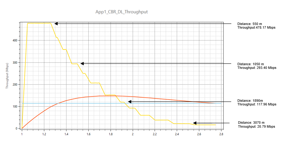
Figure 4‑51: Downlink Application Throughput Plot in LOS mode

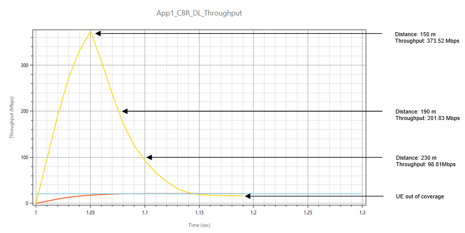
Figure 4‑52: Downlink Application Throughput Plot in NLOS mode

Uplink Line-of-Sight (LOS) and Non-Line-of-Sight (NLOS) Plots

Figure 4‑53: Uplink Application Throughput Plot in LOS mode

Figure 4‑54: Uplink Application Throughput Plot in NLOS mode

Discussion: The downlink throughput of 479.17 Mbps is maintained till \~550m in LOS whereas, it is maintained till 150m in NLOS. Similarly, the uplink throughput of 133.52 Mbps is maintained till 150m in LOS whereas, it is maintained till 130m in NLOS. The Uplink throughput falls to the lowest level at \~750m in LOS and at \~150m in NLOS.

DL: UL Ratio 3:2#

LOS and NLOS#

Step 1: All the properties were set as in DL: UL-Ratio 4:1.

Step 2: In the gNB properties-> Interface 5G_RAN, the DL:UL ratio was set to 3:2.

Step 3: The following settings were done in application properties:

Parameter	Value
APP1_CBR_DL
Source	Wired_Node_10
Destination	UE_8
Start Time (s)	1
Packet Size (Bytes)	1460
IAT (µs)	11.68
Generation Rate (Mbps)	1000
Transport Protocol	UDP
APP2_CBR_UL
Source	UE_8
Destination	Wired_Node_10
Start Time (s)	1
Packet Size (Bytes)	1460
IAT (µs)	38.93
Generation Rate (Mbps)	300
Transport Protocol	UDP

Table 4‑55: Application Properties

Step 3: Run simulation for 2.75s.

Step 4: Similarly, in LOS, set the LOS Probability to 0 in gNB properties and run simulation for 1.3s.

Results:

Downlink Line-of-Sight (LOS) and Non-Line-of-Sight (NLOS) Plots

Figure 4‑55: Downlink Application Throughput Plot in LOS mode

Figure 4‑56: Downlink Application Throughput Plot in NLOS mode

Uplink Line-of-Sight (LOS) and Non-Line-of-Sight (NLOS) Plots

Figure 4‑57: Uplink Application Throughput Plot in LOS mode

Figure 4‑58: Uplink Application Throughput Plot in NLOS mode

Inference: The downlink throughput of 359.74 Mbps is maintained till \~550m in LOS whereas, it is maintained till 130m in NLOS. Similarly, the uplink throughput of 238.50 Mbps is maintained till 130m in LOS whereas, it is 35.97 Mbps maintained till 130m in NLOS. The Uplink throughput falls to the lowest level at \~750m in LOS and at \~150m in NLOS.

Urban gNB cell radius for different data rates #

Open NetSim, Select Examples->5G NR ->gNB cell radius for different data rates then click on the tile in the middle panel to load the example as shown in below screenshot

Figure 4‑59: List of scenarios for the example of gNB cell radius for different data rates

3.5 GHz n78 urban gNB cell radius for different data rates#

The following network diagram illustrates, what the NetSim UI displays on clicking.

Figure 4‑60: Network set up for studying the gNB cell radius for different data rates

Setting done in example config file:

1. Set the following property as shown in below Table 4‑56.

gNB Properties -> Interface (5G_RAN)
gNB Height	10m
Tx Power	40
CA Type	Single Band
CA Configuration	n78
DL: UL	4:1
Numerology	2
Channel Bandwidth	50 MHz
MCS Table	QAM256
CQI Table	TABLE2
Outdoor Scenario	Urban Macro
Pathloss Model	3GPPTR38.901-7.4.1
LOS_NLOS Selection	3GPPTR38.901-Table7.4.2-1
Shadow Fading Model	None
Fading _and_Beamforming	NO_FADING_MIMO_UNIT_GAIN
O2I Building Penetration Model	None

Table 4‑56: gNB >Interface (5G_RAN) >Physical layer properties

1. Set the Tx_Antenna Count as 8 and Rx_Antenna Count as 1 in gNB> Interface 5G_RAN > Physical Layer.

2. Set the Tx_Antenna Count as 1 and Rx_Antenna Count as 8 in UE> Interface 5G_RAN > Physical Layer.

3. Set Uplink speed and Downlink speed as 100000 Mbps and BER as 0.

4. Set the following application properties:

App_1_CBR
Source Id	10
Destination Id	8
Packet Size	1460
IAT	1.94 µs
Start time	1s
Transport Protocol	UDP
Generation Rate	6 Gbps

Table 4‑57: Application properties

1. Plots are enabled in NetSim GUI.

2. Run simulation for 1.1 sec. After simulation completes go to metrics window and note down throughput value from application metrics.

Go back to the Scenario and change distance between gNB and UE to 100m, 130m, 150m, 170m, 190m, 200m, 300m, 330m, and 350m and run simulation for 1.1 sec.

Result:

Cell Radius (m)	Data Rate (Mbps). Downlink
≈1500 Mbps Downlink
100	1574.81
130	1335.72
150	1205.37
≈1000 Mbps Downlink
170	1096.75
190	955.42
200	825.07
≈500 Mbps Downlink
300	499.20
330	412.30
350	303.68

Table 4‑58: Results Comparison

26 GHz n258 urban gNB cell radius for different data rates#

Setting done in example config file:

1. Set the following property as shown in below given table:

gNB Properties -> Interface (5G_RAN)
gNB Height	10m
Tx Power	40
MCS Table	QAM256
CQI Table	TABLE2
CA Type	Single Band
CA Configuration	N258
DL: UL	4:1
Numerology	2
Channel Bandwidth	200 MHz
Outdoor Scenario	Urban Macro
Pathloss Model	3GPPTR38.901-7.4.1
LOS_NLOS Selection	3GPPTR38.901-Table7.4.2-1
Shadow Fading Model	None
Fading _and_Beamforming	NO_FADING_MIMO_UNIT_GAIN
O2I Building Penetration Model	None

Table 4‑59: gNB >Interface (5G_RAN) >Physical layer properties

1. Set the Tx_Antenna Count as 8 and Rx_Antenna Count as 1 in gNB> Interface 5G_RAN > Physical Layer.

2. Set the Tx_Antenna Count as 1 and Rx_Antenna Count as 8 in UE> Interface 5G_RAN > Physical Layer.

3. Set Uplink speed and Downlink speed as 100000 Mbps and BER as 0.

4. Set the following application properties:

App_1_CBR
Source Id	10
Destination Id	8
Packet Size	1460
IAT	1.94 µs
Start time	1s
Transport Protocol	UDP
Generation Rate	6 Gbps

Table 4‑60: Application properties

1. Plots are enabled in NetSim GUI.

2. Run simulation for 1.1 sec. After simulation completes go to metrics window and note down throughput value from application metrics.

Go back to the Scenario and change distance between gNB and UE to 20m, 110m, and 150m and run simulation for 1.1 sec.

Result:

Cell Radius (m)	Data Rate (Mbps). Downlink
≈6000 Mbps Downlink
20	5986.81
≈1000 Mbps Downlink
110	724.86
≈ 500 Mbps Downlink
150	298.07

Table 4‑61: Results Comparison

Impact of numerology on a RAN with phones, sensors, and cameras #

Open NetSim, Select Examples ->5G NR -> Impact of numerology on a RAN with phones sensors and cameras then click on the tile in the middle panel to load the example as shown in below Figure 4‑61.

Figure 4‑61: List of scenarios for the example of Impact of numerology on a RAN with phones sensors and cameras

Network Scenario[^3]: To model a real-world scenario, we base our simulation on the setup shown in Figure 4‑62. The link between the gNB and the L2_Switches that represents the Core Network (CN) is made with a point-to-point 10 Gb/s link, without propagation delay. The Radio Area Network (RAN) is served by 1 gNB, in which different UEs share the connectivity. We have 25 smartphones, 6 sensors, 3 IP cameras. The bandwidth is 100MHz and Round Robin MAC Scheduler. The position of the devices in the reference scenario depicted in Figure 4‑62 is quasi-random.

Figure 4‑62: Network set up for studying the with 25 smartphones, 6 sensors and 3 cameras communicating with respective cloud servers

In terms of application data traffic, the camera (video) and sensor nodes have one UDP flow each, that goes in the UL towards a remote node on the Internet. These flows are fixed-rate flows: we have a continuous transmission of 5 Mb/s for the video nodes, to simulate a 720p24 HD video, and the sensors transmit a payload of 500 bytes each 2.5 ms, that gives a rate of 1.6 Mb/s. For the smartphones, we use TCP as the transmission protocol. These connect to data base servers. Each phone has to download a 25 MB file and to upload one file of 1.5 MB. These flows start at different times: the upload starts at a random time between the 25^th and the 75^th simulation seconds, while each download starts at a random time between the 1.5^th and the 95^th simulation seconds.

	Flows (No of devices)	Traffic Rate (Mbps)	Segment / File Size (B)	RAN Dir.	TCP ACK Dir.
Camera (UDP)	3	5	500	UL	-
Sensor (UDP)	6	1.6	500	UL	-
Smartphone Upload (TCP)	25	-	1,500,000	UL	DL
Smartphone Download (TCP)	25	-	25,000,000	DL	UL

Table 4‑62: Various parameters of the Traffic flow models for all the devices

The numerology  μ can take values from 0 to 3 and specifies an SCS of 15 × 2^μ kHz and a slot length of $\frac{1}{2^{\mu}}$ ms. FR1 support μ = 0, 1 and 2, while FR2 supports μ = 2, 3. We study the impact of different numerologies, and how they affect the end-to-end performance. The metrics measured and analysed are a) Throughput of TCP uploads & downloads, and b) Latency of the UDP uploads

Settings done in example config file:

1. For the above scenario set the following given properties:

gNB Properties -> Interface (5G_RAN)
Pathloss Model	None
Frequency Range	FR1
CA Type	Inter Band CA
CA_Configuration	CA_2DL_2UL_n40_n41
CA1
Numerology	0, 1, and 2
Channel Bandwidth	50 MHz
DL_UL Ratio	1:4
CA2
Numerology	0, 1, and 2
Channel Bandwidth	50 MHz
DL_UL Ratio	1:4
MCS Table	QAM64
CQI Table	TABLE1

Table 4‑63: gNB >Interface (5G_RAN) >Physical layer properties

Link Properties (All wired links)
Uplink/ Downlink Speed (Mbps)	10000
Uplink/ Downlink BER	0
Uplink/ Downlink Propagation Delay (μs)	5

Table 4‑64: Wired Link Properties

1. The following Application properties set to the above scenario:

Sensor UL UDP
Generation Rate (Mbps)	1.6
Transport Protocol	UDP
Application Type	Custom
Packet Size (Bytes)	500
Inter Arrival Time (μs)	2500

Table 4‑65: Sensor Application Properties for UL UDP

Camera UL UDP
Generation Rate (Mbps)	5
Transport Protocol	UDP
Application Type	Custom
Packet Size (Bytes)	500
Inter Arrival Time (μs)	800

Table 4‑66: Camera Application Properties for UL UDP

Phone DL TCP
Transport Protocol	TCP
Start Time (s)	1.5  + 4(t), Where, i = 0, 1, 2, ……, 48
Stop Time (s)	95
File Size (Bytes)	25,000,000
Inter Arrival Time (s)	200 (Simulation ends at 100s and hence only one file is sent)
Application Type	FTP

Table 4‑67: Phone Application Properties for DL TCP

Phone UL TCP
Application Type	FTP
Transport Protocol	TCP
Start Time (s)	\[25 + 2(i - 1)\ \] Where, \(i = 1,\ 2,\ldots\ldots,\ 25\)
Stop Time (s)	95
File Size (Bytes)	1,500,000
Inter Arrival Time (s)	200 (Simulation ends at 100s and hence only one file is sent)

Table 4‑68: Phone Application Properties for UL TCP

1. The Tx_Antenna_Count was set to 2 and Rx_Antenna_Count was set to 4 in gNB > Interface 5G_RAN >Physical Layer.

2. The Tx_Antenna_Count was set to 4 and Rx_Antenna_Count was set to 2 in UE > Interface 5G_RAN >Physical Layer.

3. Run simulation for 100 sec. After simulation completes go to metrics window and note down throughput and delay value from application metrics.

Result and Analysis:

Numerology(μ) = 0
Camera Uplink		Sensor Uplink		Smartphone
				Uplink	Downlink
Throughput (Mbps)	Delay (μs)	Throughput (Mbps)	Delay (μs)	Throughput (Mbps)	Throughput (Mbps)
4.99	1845.51	1.6	2274.02	89.80	0.00
4.99	1848.21	1.6	2272.62	89.80	0.00
4.99	1850.91	1.6	2279.64	89.80	0.00
		1.6	2278.24	89.80	0.00
		1.6	2276.83	89.80	0.00
		1.6	2275.43	89.80	0.00
				89.80	0.00
				89.80	0.00
				89.80	0.00
				89.80	80.50
				89.80	85.69
				90.00	75.43
				3.62	86.27
				0.23	86.26
				0.35	86.27
				0.17	86.27
				0.27	86.27
				0.36	86.27
				1.35	86.27
				1.51	86.27
				0.69	86.27
				2.36	86.27
				2.34	86.27
				1.85	86.27
				1.39	86.27

Table 4‑69: Throughput and delay for Camera, Sensors and Smartphones, When μ = 0

Numerology(μ) = 1
Camera Uplink		Sensor Uplink		Smartphone
				Uplink	Downlink
Throughput (Mbps)	Delay (μs)	Throughput (Mbps)	Delay (μs)	Throughput (Mbps)	Throughput (Mbps)
4.99	35801.94	1.60	1523.71	154.02	0.00
4.99	35720.37	1.60	1522.31	154.02	0.00
4.99	35948.59	1.60	1529.32	154.02	0.00
		1.60	1527.92	154.02	0.00
		1.60	1526.52	154.02	0.00
		1.60	1525.11	154.02	0.00
				154.02	0.00
				154.02	0.00
				154.02	0.00
				154.02	0.00
				154.02	172.52
				154.02	172.52
				153.72	171.37
				0.52	171.37
				0.54	171.37
				0.66	171.37
				0.63	171.37
				0.68	171.37
				4.56	171.37
				7.14	171.37
				6.61	171.37
				1.11	171.37
				5.58	171.37
				5.68	171.37
				2.09	171.37

Table 4‑70: Throughput and delay for Camera, Sensors and Smartphones, When μ=

1

Numerology(μ) = 2
Camera Uplink		Sensor Uplink		Smartphone
				Uplink	Downlink
Throughput (Mbps)	Delay (μs)	Throughput (Mbps)	Delay (μs)	Throughput (Mbps)	Throughput (Mbps)
5.00	78284.10	1.60	773.57	149.33	0.00
5.00	79995.75	1.60	772.17	149.33	0.00
5.00	52688.39	1.60	779.18	149.33	0.00
		1.60	777.78	149.33	0.00
		1.60	776.38	149.33	0.00
		1.60	774.97	149.33	0.00
				149.33	0.00
				149.33	0.00
				149.33	0.00
				149.33	0.00
				149.33	344.74
				149.33	344.73
				149.33	342.61
				4.62	342.61
				4.63	342.61
				5.50	342.61
				6.60	342.61
				8.56	342.61
				10.32	342.61
				11.48	342.61
				11.46	342.61
				11.41	342.61
				11.44	342.61
				11.44	342.61
				11.40	342.61

Table 4‑71: Throughput and delay for Camera, Sensors and Smartphones, When μ = 2

Figure 4‑63: The average uplink throughput for camera and sensors remains the same as numerology is increased. This is because the flow is UDP.

Figure 4‑64: Smartphone Uplink, and Smartphone Downlink average throughput vs. Numerology (µ)

Figure 4‑65: Camera Uplink, and Sensor Uplink Latency vs. Numerology. The latency drops as the numerology increases

For UDP applications the μ does not impact the throughput. However, higher μ leads to an obviously lower delay. The variation of delay vs. μ is as follows:

	Avg Delay (Camera)	Avg Delay (Sensor)
μ = 0	1.838 ms	2.286 ms
μ = 1	0.930 ms	1.536 ms
μ = 2	0.476 ms	0.780 ms

Table 4‑72: Variation of delay vs. numerology for Camera and Sensors

The TCP throughput is inversely proportional to round trip time. Therefore, for applications running over TCP the throughput increases with higher numerology. This is because higher Numerology leads to reduced round-trip (end-to-end) times.

Impact of UE movement on Throughput #

Open NetSim, Select Examples ->5G NR -> UE Movement vs Throughput then click on the tile in the middle panel to load the example as shown in below Figure 4‑66.

Figure 4‑66: List of scenarios for the example of UE Movement vs Throughput

NetSim UI displays the configuration file corresponding to this experiment as shown below in Figure 4‑67.

Figure 4‑67: Network set up for studying Throughput vs. UE Movement

The following set of procedures were done to generate this sample:

Step 1: A network scenario is designed in NetSim GUI comprising of 1 gNB, 5G-Core, and 1 UE and 1 Wired Node in the “5G NR” Network Library.

Step 2: Grid Length was set to 5100 m x 5100 m.

Step 3: The device positions are set as per the table given below Table 4‑73.

Device	UE_8	gNB_7	Wired_Node_10
x- axis	500	500	3500
y- axis	1	0	1020

Table 4‑73: Device general properties

Step 4: The following properties were set in Interface (5G_RAN) of gNB

Parameter	Value
Tx_Power	40
gNB Height	10m
CA Type	Single Band
CA Configuration	n78
DL-UL Ratio	4:1
Numerology	0
Channel Bandwidth	10 MHz
MCS Table	QAM64LOWSE
CQI Table	TABLE3
Propagation Model	Urban Macro
Pathloss Model	3GPPTR38.901-7.4.1
LOS_NLOS_Selection	User Defined
LOS Probability	0
Shadow Fading Model	None
Fading and Beamforming	NO_FADING_MIMO_UNIT_GAIN
O2I Building Penetration Model	Low Loss Model

Table 4‑74: gNB >Interface (5G_RAN) >Physical layer properties

Step 5: Set Tx_Antenna_Count and Rx_Antenna_Count as 2 and 1 in gNB properties > Interface(5G_RAN) > Physical Layer.

Step 6: Set Tx_Antenna_Count and Rx_Antenna_Count as 1 and 2 in UE properties > Interface(5G_RAN) > Physical Layer.

Step 7: In the General Properties of UE 8, set Mobility Model as File Based Mobility

Step 8: A CBR Application was generated from Wired Node 10 i.e. Source to UE 8 i.e. Destination with Packet Size remaining 1460Bytes and Inter Arrival Time remaining 1168µs.

Step 9: The Transport Protocol was set to UDP.

Step 10: Additionally, the “Start Time(s)” parameter is set to 1s, while configuring the application.

File Based Mobility: In File Based Mobility, users can write their own custom mobility models and define the movement of the mobile users. Create a mobility.txt file for UE’s involved in mobility with each step equal to 4 sec with distance 100 m.

The NetSim Mobility File (mobility.txt) format is as follows:

$time 0.0 "$node_(7) 500.0 1.0 0.0"

$time 4.0 "$node_(7) 500.0 101.0 0.0"

$time 8.0 "$node_(7) 500.0 201.0 0.0"

$time 12.0 "$node_(7) 500.0 301.0 0.0"

$time 16.0 "$node_(7) 500.0 401.0 0.0"

$time 20.0 "$node_(7) 500.0 501.0 0.0"

$time 24.0 "$node_(7) 500.0 601.0 0.0"

$time 28.0 "$node_(7) 500.0 701.0 0.0"

$time 32.0 "$node_(7) 500.0 801.0 0.0"

$time 36.0 "$node_(7) 500.0 901.0 0.0"

$time 40.0 "$node_(7) 500.0 1001.0 0.0"

$time 44.0 "$node_(7) 500.0 1101.0 0.0"

$time 48.0 "$node_(7) 500.0 1201.0 0.0"

$time 52.0 "$node_(7) 500.0 1301.0 0.0"

$time 56.0 "$node_(7) 500.0 1401.0 0.0"

$time 60.0 "$node_(7) 500.0 1501.0 0.0"

$time 64.0 "$node_(7) 500.0 1601.0 0.0"

$time 68.0 "$node_(7) 500.0 1701.0 0.0"

$time 72.0 "$node_(7) 500.0 1801.0 0.0"

$time 76.0 "$node_(7) 500.0 1901.0 0.0"

$time 80.0 "$node_(7) 500.0 2001.0 0.0"

$time 84.0 "$node_(7) 500.0 2101.0 0.0"

$time 88.0 "$node_(7) 500.0 2201.0 0.0"

$time 92.0 "$node_(7) 500.0 2301.0 0.0"

$time 96.0 "$node_(7) 500.0 2401.0 0.0"

$time 100.0 "$node_(7) 500.0 2501.0 0.0"

Step 11: Plots is enabled in NetSim GUI.

Step 12: Run simulation for 100s.

Results:

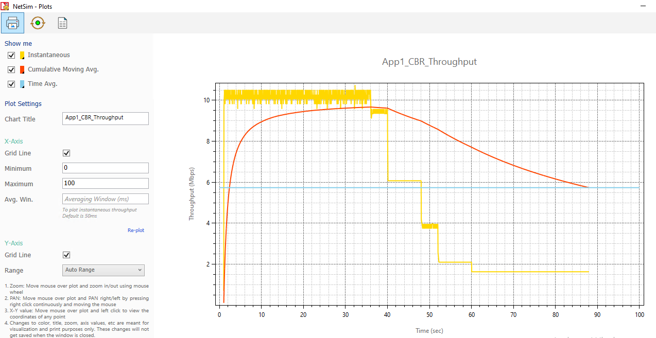
Figure 4‑68: Plot of Throughput (Mbps) vs Time (sec)

Discussion

As the UE moves away from the gNB, the Application throughput starts reducing. The maximum throughput of 10 Mbps is obtained until 40 sec. At 40s the UE is 1000m away from the gNB. Then the throughput drops to 9.3 Mbps at 40 sec and at time 48 sec (when UE is 1200m away from gNB), the throughput drops to 6 Mbps and at time 52 sec (when UE is 1300m away from gNB), the throughput drops to 3.26 Mbps and subsequently keeps dropping as till the end of the simulation as the UE continues to move further away from the gNB.

.