Transmission control protocol (TCP)

Introduction to TCP connection management (Level 1)

Introduction

When an application process in a client host seeks a reliable data connection with a process in another host (say, server), the client-side TCP then proceeds to establish a TCP connection with the TCP at the server side. A TCP connection is a point-to-point, full-duplex logical connection with resources allocated only in the end hosts. The TCP connection between the client and the server is established in the following manner and is illustrated in Figure-1.

The TCP at the client side first sends a special TCP segment, called the SYN packet, to the TCP at the server side.
Upon receiving the SYN packet, the server allocates TCP buffer and variables to the connection. Also, the server sends a connection-granted segment, called the SYN-ACK packet, to the TCP at the client side.
Upon receiving the SYN-ACK segment, the client also allocates buffers and variables to the connection. The client then acknowledges the server’s connection granted segment with an ACK of its own.

This connection establishment procedure is often referred to as the three-way handshake. The special TCP segments can be identified by the values in the fields SYN, ACK and FIN in the TCP header (see Figure-2). We also note that the TCP connection is uniquely identified by the source and destination port numbers (see Figure-2) exchanged during TCP connection establishment and the source and destination IP addresses.

Once a TCP connection is established, the application processes can send data to each other. The TCP connection can be terminated by either of the two processes. Suppose that the client application process seeks to terminate the connection. Then, the following handshake ensures that the TCP connection is torn down.

The TCP at the client side sends a special TCP segment, called the FIN packet, to the TCP at the server side.
When the server receives the FIN segment, it sends the client an acknowledgement segment in return and its own FIN segment to terminate the full-duplex connection.
Finally, the client acknowledges the FIN-ACK segment (from the server) with an ACK of its own. At this point, all the resources (i.e., buffers and variables) in the two hosts are deallocated.

During the life of a TCP connection, the TCP protocol running in each host makes transitions through various TCP states. Figure-1 illustrates the typical TCP states visited by the client and the server during connection establishment and data communication.

TCP is defined in RFCs 793, 1122, 7323 and, 2018. A recommended textbook reference for TCP is Chapter 3: Transport layer, of Computer Networking: A top-down approach, by James Kurose and Keith Ross (Pearson).

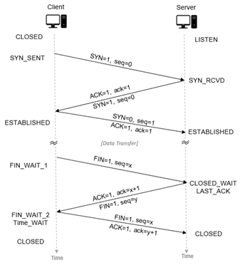
Figure-1: TCP connection establishment between a client and a server

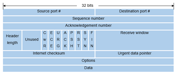
Figure-2: TCP Header

Network Setup

Open NetSim and click on Experiments >Internetworks> TCP> Introduction to TCP connection management then click on the tile in the middle panel to load the example as shown in below Figure-3.

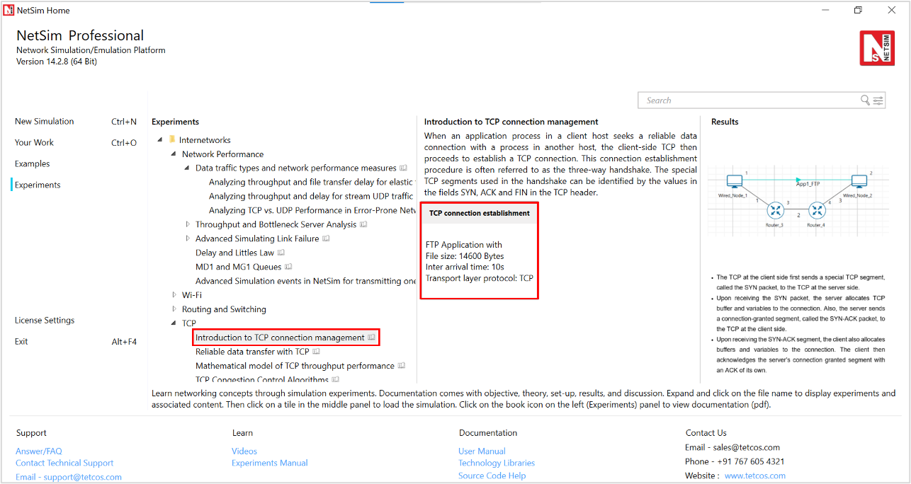
Figure-3: List of scenarios for the example of Introduction to TCP connection management

NetSim UI displays the configuration file corresponding to this experiment as shown below Figure-4

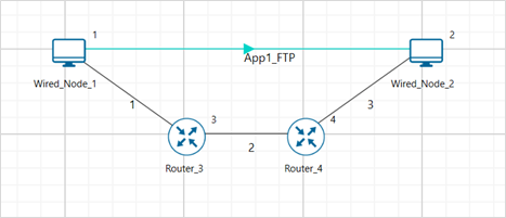
Figure-4: Network set up for studying the Introduction to TCP connection management

Procedure

The following set of procedures were done to generate this sample.

Step 1: A network scenario is designed in NetSim GUI comprising of 2 Wired Nodes and 2 Routers in the “Internetworks” Network Library.

Step 2: In the General Properties of Wired Node 1 i.e., Source, Wireshark Capture is set to Online. Transport Layer properties Congestion Control algorithm set to NEW RENO.

To configure any properties in the nodes, click on the node, expand the property panel on the right side, and change the properties as mentioned in the steps.

NOTE: Routers are configured with default properties.

Step 3: Click on the link ID (of a wired link) and expand the link property panel on right. Set Max Uplink Speed and Max Downlink Speed to 10 Mbps. Set Uplink BER and Downlink BER to 0. Set Uplink Propagation Delay and Downlink Propagation Delay as 100 microseconds for the links 1 and 3 (between the Wired Node’s and the routers). Set Uplink Propagation Delay and Downlink Propagation Delay as 50000 microseconds for the backbone link connecting the routers, i.e., 2.

Step 4: Configure FTP application between two nodes by selecting an application from the Set Traffic tab in the ribbon at the top. Click on the application flow App1 FTP, expand the application properties panel on the right, and set the File Size set to 14600 Bytes and File Inter Arrival Time set to 10 Seconds

Step 5: Click on Show/Hide info > Device IP check box in the NetSim GUI to view the network topology along with the IP address.

Step 6: Enable the Throughput vs Time plots under Link and Application performance and Run simulation for 10 seconds.

Output

We have enabled Wireshark capture in Wired Node 1. The PCAP file is generated at the end of the simulation and is shown in Figure-5.

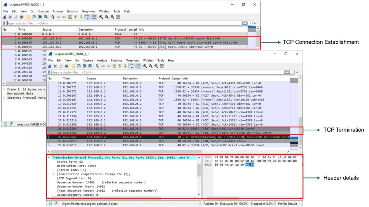
Figure-5: Wireshark Packet capture at Wired Node 1

The 3-way handshake of TCP connection establishment and TCP connection termination is observed in the packet capture (Figure 4 5).
Data is transferred only after the TCP connection is established.
We can access the packet header details of the TCP segments (SYN, SYN-ACK, FIN, FINACK) in Wireshark.

Note that:

When devices in different Wide Area Networks (WANs) need to communicate, their private IP addresses are converted to public IP addresses using Network Address Translation (NAT). In the above TCP sample, WireShark captures the TCP three-way handshake as shown in Figure 4 5. Here the source device in one network (192.168.0.2) sends data to another network via Router 3.
Router 3 converts its private IP (192.168.0.1) to a public one (11.0.0.3) using NAT, allowing it to communicate with devices outside its network.
The data is then forwarded to Router 4 in another network, where NAT converts the public IP (11.0.0.2) back to a private one (192.169.0.1) to reach the destination device (192.169.0.2).
This process enables communication between devices in different networks using public IP addresses, while devices within the same network can communicate using their private IP addresses.

Exercises

Construct a scenario with 2 nodes and 2 routers. Introduce the link failure and recovery at Router3. Set Uptime as 0, 10, and the downtime as 5. This means the link is up from 0s – 5s, then down from 5s - 10s and then up again after 10s. Explain what you observe in between 5th second and 10th second using the packet trace. Does TCP reestablish connection after 10s?

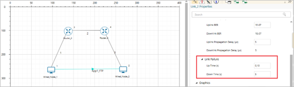
Figure-6: Network scenario for TCP.

For more variations change the number of routers, link speeds, and the time at which the link fails and recovers.

Reliable data transfer with TCP (Level 1)

Introduction

TCP provides reliable data transfer service to the application processes even when the underlying network service (IP service) is unreliable (loses, corrupts, garbles or duplicates packets). TCP uses checksum, sequence numbers, acknowledgements, timers and retransmission to ensure correct and in order delivery of data to the application processes.

TCP views the data stream from the client application process as an ordered stream of bytes. TCP will grab chunks of this data (stored temporarily in the TCP send buffer), add its own header and pass it on to the network layer. A key field of the TCP header is the sequence number which indicates the position of the first byte of the TCP data segment in the data stream. The sequence number will allow the TCP receiver to identify segment losses, duplicate packets and to ensure correct delivery of the data stream to the server application process.

When a server receives a TCP segment, it acknowledges the same with an ACK segment (the segment carrying the acknowledgement has the ACK bit set to 1) and also conveys the sequence number of the first missing byte in the application data stream, in the acknowledgement number field of the TCP header. All acknowledgements are cumulative; hence, all missing, and out-of-order TCP segments will result in duplicate acknowledgements for the corresponding TCP segments.

TCP sender relies on sequence numbering and acknowledgements to ensure reliable transfer of the data stream. In the event of a timeout (no acknowledgement is received before the timer expires) or triple duplicate acknowledgements (multiple ACK segments indicate a lost or missing TCP segment) for a TCP segment, the TCP sender will retransmit the segment until the TCP segment is acknowledged (at least cumulatively). In Figure-7, we illustrate retransmission by the TCP sender after a timeout for acknowledgement.

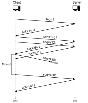
Figure-7: An illustration of TCP retransmission with timeout. The segment with sequence number 4381 is lost in the network. The TCP client retransmits the segment after a timeout event.

Network Setup

Open NetSim and click on Experiments > Internetworks> TCP> Reliable data transfer with TCP then click on the tile in the middle panel to load the example as shown in below Figure-8.

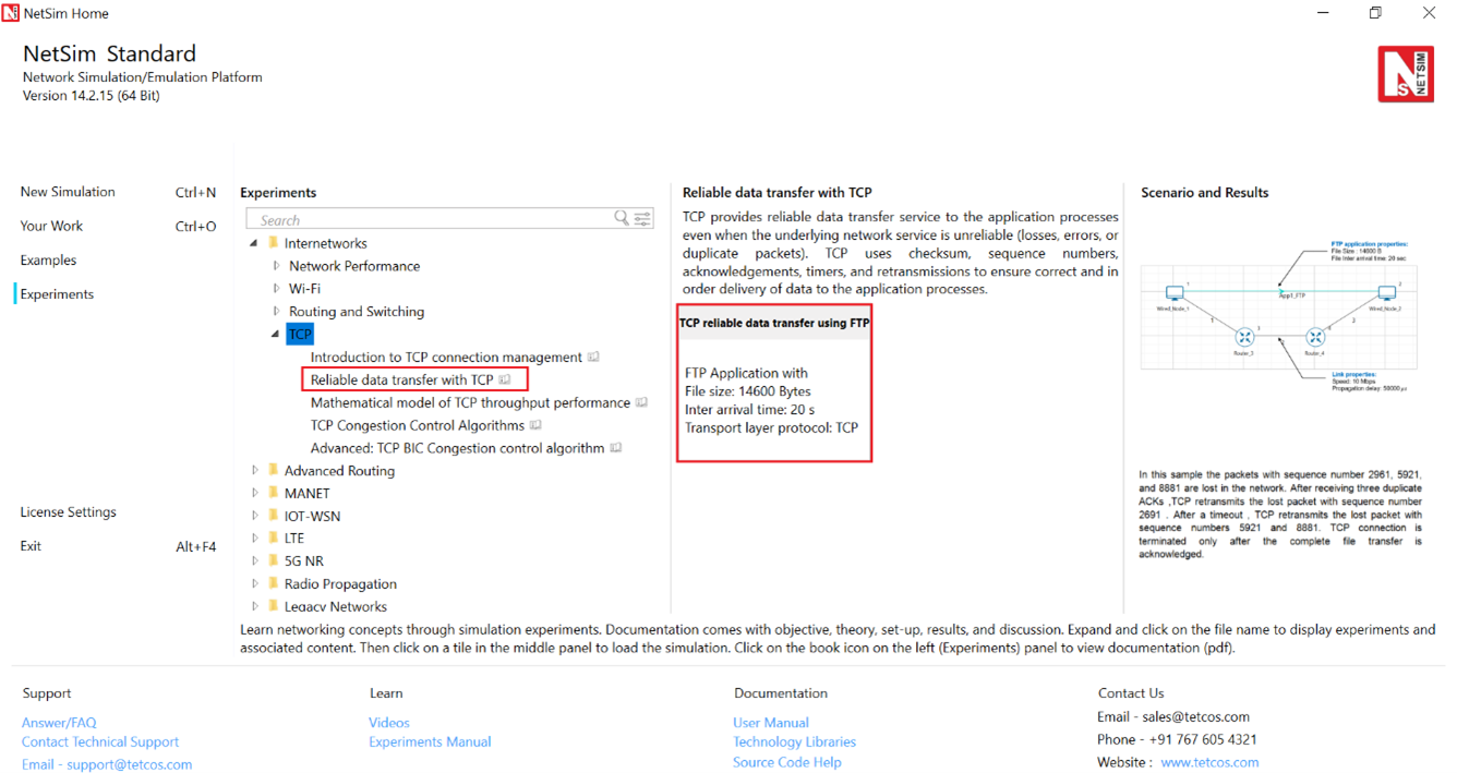
Figure-8: List of scenarios for the example of Reliable data transfer with TCP

NetSim UI displays the configuration file corresponding to this experiment as shown below Figure-9.

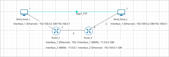
Figure-9: Network set up for studying the Reliable data transfer with TCP

We will seek a simple file transfer with TCP over a lossy link to study reliable data transfer with TCP. We will simulate the network setup illustrated in Figure-9 with the configuration parameters listed in detail to study reliable data transfer with TCP connection.

Procedure

The following set of procedures were done to generate this sample.

Step 1: A network scenario is designed in NetSim GUI comprising of 2 Wired Nodes and 2 Routers in the “Internetworks” Network Library.

Step 2: In the General Properties of Wired Node 1 i.e., Source and Wired Node 2 i.e., Destination, Wireshark Capture is set to Online.

To configure any properties in the nodes, click on the node, expand the property panel on the right side, and change the properties as mentioned in the steps.

Note: Routers are configured with default properties.

Step 3: Click on the link ID (of a wired link) and expand the link properties panel on right. Set Max Uplink Speed and Max Downlink Speed to 10 Mbps. Set Uplink BER and Downlink BER to 0. Set Uplink Propagation Delay and Downlink Propagation Delay as 100 microseconds for the links 1 and 3 (between the Wired Node’s and the routers). Set Uplink Propagation Delay and Downlink Propagation Delay as 50000 microseconds and Uplink BER and Downlink BER to 0.00001 for the backbone link connecting the routers, i.e., 2.

Step 4: Configure FTP application between two nodes by selecting an application from the Set Traffic tab in the ribbon at the top. Click on the application flow App1 FTP, expand the application properties panel on the right, and set the File Size to 14600 bytes and the File Inter Arrival Time to 20 seconds.

Step 5: Click on Show/Hide info > Enable Device IP check box in the NetSim GUI to view the network topology along with the IP address.

Step 6: Enable Throughput vs Time plots under Application and link performance and click on Run simulation. The simulation time is set to 20 seconds.

Output

We aimed to transfer a file of size 14600 bytes (i.e., 10 packets, each of size 1460 bytes) with TCP over a lossy link. In Figure-10, we report the application metrics data for FTP which indicates that the complete file was transferred.

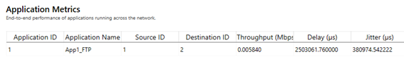
Figure-10: Application Metrics table for FTP

We have enabled Wireshark Capture in Wired Node 1 and Wired Node 2. The PCAP files are generated at the end of the simulation and are shown in Figure-11 and Figure-12.

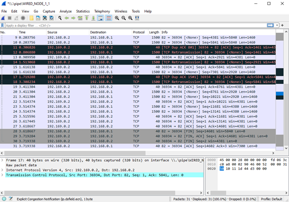
Figure-11: PCAP file at Wired Node 1. TCP ensures reliable data transfer using timeout, duplicate ACKs and retransmissions.

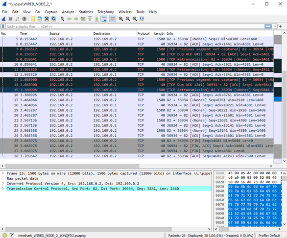
Figure-12: PCAP file at Wired Node 2

Inference

From Figure-11 and Figure-12, we note that the packets with sequence number 1461 and 5841 are errored in the network, which can also observe in Packet Trace.
After receiving three duplicate ACKs (in lines 13, 14 of Figure-11), TCP retransmits the errored packet. (In line 15 of Figure-11).
TCP connection is terminated only after the complete file transfer is acknowledged which can be observed in Figure-5 (Line 25 and 26).

Mathematical Modelling of TCP Throughput Performance (Level 2)

Introduction

The average throughput performance of additive-increase multiplicative-decrease TCP congestion control algorithms have been studied in a variety of network scenarios. In the regime of large RTT, the average throughput performance of the TCP congestion control algorithms can be approximated by the ratio of the average congestion window cwnd and RTT.

Loss-less Network

In a loss-less network, we can expect the TCP congestion window cwnd to quickly increase to the maximum value of 64 KB (without TCP scaling). In such a case, the long-term average throughput of TCP can be approximated as

\[Throughput\ \approx \frac{64 \times 1024\ (bits)}{RTT\ (in\ secs)}\]

Lossy Network

We refer to an exercise in Chapter 3 of Computer Networking: A top-down approach, by Kurose and Ross for the setup. Consider a TCP connection over a lossy link with packet error rate p. In a period of time between two packet losses, the congestion window may be approximated to increase from an average value of W/2 to W (see Figure-20 for motivation). In such a scenario, the throughput can be approximated to vary from W/2/RTT to W/RTT (in the cycle between two packet losses). Under such assumptions, we can then show that the loss rate (fraction of packets lost) must be equal to

\[p = \frac{1}{\frac{3}{8}W^{2} + \frac{3}{4}W}\]

and the average throughput is then approximately,

\[Throughput \approx \sqrt{\frac{3}{2p}\ } \times \frac{MSS\ (in\ bits)}{RTT\ (in\ secs)}\]

Network Setup

Open NetSim and click on Experiments> Internetworks> TCP> Mathematical model of TCP throughput performance then click on the tile in the middle panel to load the example as shown below in Figure-13.

Figure-13: List of scenarios for the example of Mathematical model of TCP throughput performance

NetSim UI displays the configuration file corresponding to this experiment as shown below Figure-14.

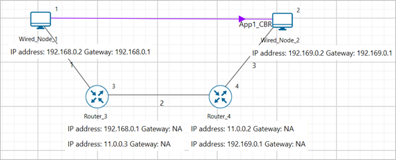
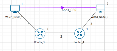
Figure-14: Network set up for studying the Mathematical model of TCP throughput performance

We will seek a large file transfer with TCP over a loss-less and lossy link to study long-term average throughput performance of the TCP congestion control algorithm. We will simulate the network setup illustrated in Figure-14 with the two (loss-less and lossy) configuration parameters listed in detail to study the throughput performance of TCP New Reno.

Procedure

Packet Loss Probability with BER-0 Sample

The following set of procedures were done to generate this sample.

Step 1: A network scenario is designed in NetSim GUI comprising of 2 Wired Nodes and 2 Routers in the “Internetworks” Network Library.

Step 2: In the General Properties of Wired Node 1 i.e., Source, Wireshark Capture is set to Online. Transport Layer properties Congestion Control algorithm is set to NEW RENO.

To configure any properties in the nodes, click on the node, expand the property panel on the right side, and change the properties as mentioned in the steps.

NOTE: Routers are configured with default properties.

Step 3: Click the link ID (of a wired link) and expand the link properties panel on the right. Set Max Uplink Speed and Max Downlink Speed to 10 Mbps. Set Uplink BER and Downlink BER to 0. Set Uplink Propagation Delay and Downlink Propagation Delay as 100 microseconds for the links 1 and 3 (between the Wired Node’s and the routers). Set Uplink Propagation Delay and Downlink Propagation Delay as 50000 microseconds for the backbone link connecting the routers, i.e., 2.

Step 4: Configure an application between two nodes by selecting an application from the Set Traffic tab in the ribbon at the top. Click on the application flow App1 CBR, expand the application properties panel on the right, and set the Packet Size to 1460 bytes and the Inter Arrival Time to 1168 microseconds.

Step 5: Click on Show/Hide info > Device IP Enable check box in the NetSim GUI to view the network topology along with the IP address.

Step 6: Enable Application throughput vs time plot from NetSim UI. This enables us to view the throughput plot of the application App1 CBR.

Step 7: Click on Run simulation. The simulation time is set to 100 seconds.

Packet Loss Probability with BER-0.0000001 Sample

Step 1: Click the link ID (of a wired link) and expand the link properties panel on the right. Set Max Uplink Speed and Max Downlink Speed to 10 Mbps. Set Uplink BER and Downlink BER to 0. Set Uplink Propagation Delay and Downlink Propagation Delay as 100 microseconds for the links 1 and 3 (between the Wired Node’s and the routers). Set Uplink Propagation Delay and Downlink Propagation Delay as 50000 microseconds and Uplink BER and Downlink BER to 0.0000001 for the backbone link connecting the routers, i.e., 2.

Step 2: Click on Run simulation. The simulation time is set to 100 seconds.

Output

In Figure-15, we report the application metrics data for data transfer over a loss-less link (Packet Loss Probability with BER-0 sample).

Figure-15: Application Metrics with BER = 0

In Figure-16, we report the plot of long-term average throughput of the TCP connection over the loss-less link.

Set average window size to 100 ms and plot the graph.

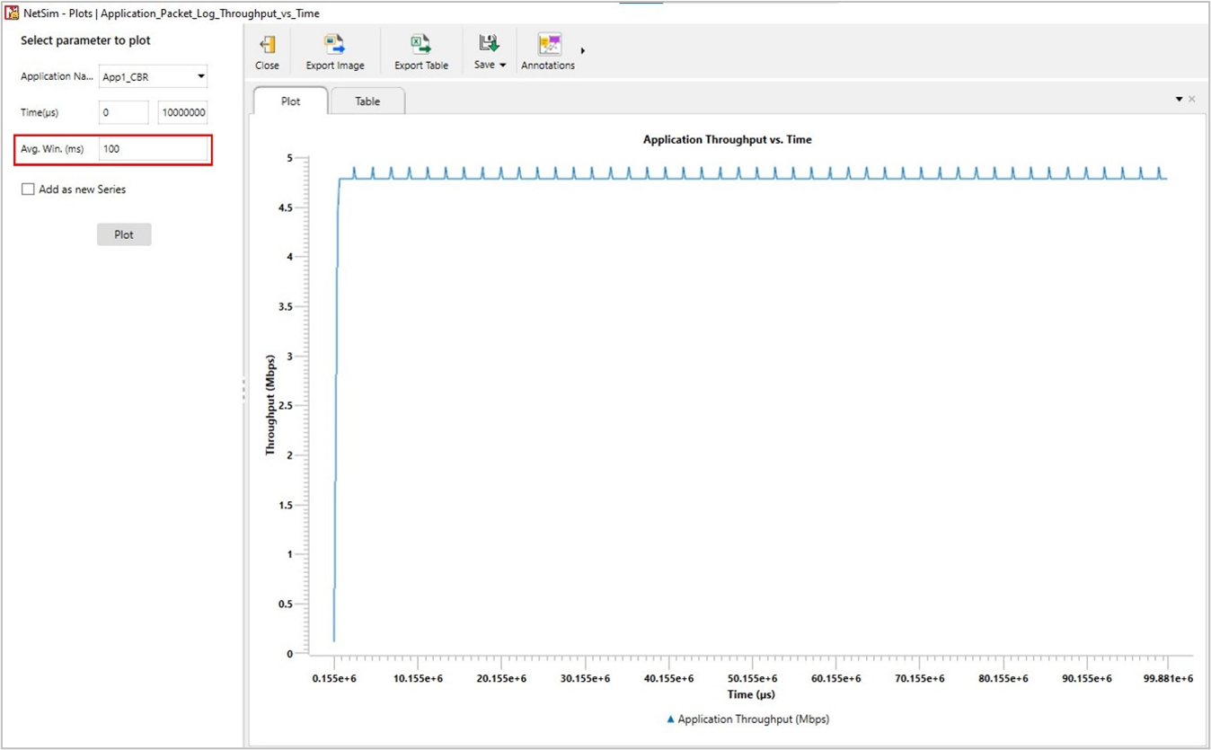
Figure-16: Long-term average throughput of TCP New Reno over a loss-less link

We have enabled Wireshark Capture in the Wired Node 1. The PCAP file is generated at the end of the simulation. From the PCAP file, the congestion window evolution graph can be obtained as follows. In Wireshark, select any data packet with a left click, then, go to Statistics > TCP Stream Graphs > Window Scaling. In Figure-17, we report the congestion window evolution of TCP New Reno over the loss-less link.

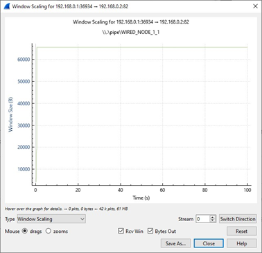
Figure-17: Congestion window evolution with TCP New Reno over a loss-less link.

In Figure-18, we report the application metrics data for data transfer over a lossy link (Packet Loss Probability with BER-0.0000001 sample).

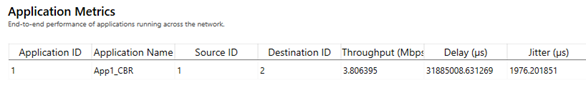
Figure-18: Application Metrics when \( \mathbf{BER = 1 \times 10^{-7}} \)

In Figure-19, we report the plot of long-term average throughput of the TCP connection over the lossy link.

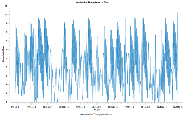
Figure-19: Throughput graph

In Figure-20, we report the congestion window evolution of TCP New Reno over the lossy link.

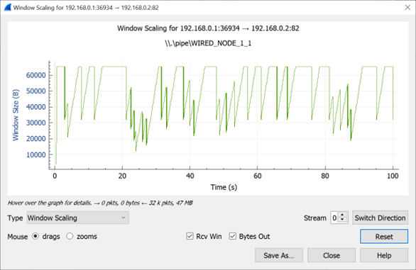
Figure-20: Congestion window evolution with TCP New Reno over a lossy link

Observations and Inference

In Figure-17, we notice that the congestion window of TCP (over the loss-less link) increases monotonically to 64 KB and remains there forever. So, a block of 64 KBs of data is transferred over a round-trip time (RTT) of approximately 100 milliseconds. Hence, a good approximation of the TCP throughput over the loss-less link is

\[Throughput \approx \frac{Window\ Size\ (in\ bits)}{RTT\ (in\ secs)}\]

\[\ \ \ \ \ \ \ \ \ \ \ \ \ \ \ \ \ \ \ \ \ \ \ \ \ \ \ \ \ \ \ \ = \frac{65535 \times 8}{100 \times 10^{- 3}} = 5.24\ Mbps\]

We note that the observed long-term average throughput (see Figure‑15) is approximately equal to the above computed value.

In Figure‑20, for the lossy link with \(BER = 1e^{- 7}\), we report the congestion window evolution with New Reno congestion control algorithm. The approximate throughput of the TCP New Reno congestion control algorithm for a packet error rate p, TCP segment size MSS and round-trip time RTT

\[Throughput \approx \sqrt{\frac{3}{2p}\ } \times \frac{MSS\ (in\ bits)}{RTT\ (in\ secs)}\]

\[\ \ \ \ \ \ \ \ \ \ \ \ \ \ \ \ \ \ \ \ \ \ \ \ \ \ \ \ \ \ \ \ \ \ \ \ \ \ \ \ \approx \sqrt{\frac{3}{2 \times 1.2 \times 10^{- 3}}} \times \frac{1460 \times 8}{100 \times 10^{- 3}}\]

\[= 4.12\ Mbps\]

where the packet error rate p can be computed from the bit error rate (\(BER = 1e^{- 7}\)) and the PHY layer packet length (1500 bytes, see packet trace) as

\[p = 1 - (1 - BER)^{1500 \times 8} \approx 1.2e^{- 3}\]

We note that the observed long-term average throughput (see Figure‑18) is approximately equal to the above computed value.

TCP Congestion Control Algorithms (Level 2)

Introduction

A key component of TCP is end-to-end congestion control algorithm. The TCP congestion control algorithm limits the rate at which the sender sends traffic into the network based on the perceived network congestion. The TCP congestion control algorithm at the sender maintains a variable called congestion window, commonly referred as cwnd, that limits the amount of unacknowledged data in the network. The congestion window is adapted based on the network conditions, and this affects the sender’s transmission rate. The TCP sender reacts to congestion and other network conditions based on new acknowledgements, duplicate acknowledgements and timeouts. The TCP congestion control algorithms describe the precise manner in which TCP adapts cwnd with the different events.

The TCP congestion control algorithm has three major phases (a) slow-start, (b) congestion avoidance, and (c) fast recovery. In slow-start, TCP is aggressive and increases cwnd by one MSS with every new acknowledgement. In congestion avoidance, TCP is cautious and increases the cwnd by one MSS per round-trip time. Slow-start and congestion avoidance are mandatory components of all TCP congestion control algorithms. In the event of a packet loss (inferred by timeout or triple duplicate acknowledgements), the TCP congestion control algorithm reduces the congestion window to 1 (e.g., Old Tahoe, Tahoe) or by half (e.g., New Reno). In fast recovery, TCP seeks to recover from intermittent packet losses while maintaining a high congestion window. The new versions of TCP, including TCP New Reno, incorporate fast recovery as well. Figure-21 presents a simplified view of the TCP New Reno congestion control algorithm highlighting slow-start, congestion avoidance and fast recovery phases.

TCP congestion control algorithm is often referred to as additive-increase multiplicative-decrease (AIMD) form of congestion control. The AIMD congestion control algorithm often leads to a “saw tooth” evolution of the congestion window (with linear increase of the congestion window during bandwidth probing and a multiplicative decrease in the event of packet losses), see Figure-26.

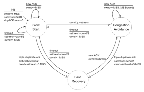
Figure-21: A simplified view of FSM of the TCP New Reno congestion control algorithm

Network Setup

We will seek a large file transfer with TCP over a lossy link to study the TCP congestion control algorithms. We will simulate the network setup illustrated in Figure-23 with the configuration parameters listed in detail in steps to study the working of TCP congestion control algorithms.

Open NetSim and click on Experiments> Internetworks>TCP> TCP Congestion Control Algorithms > Old-Tahoe then click on the tile in the middle panel to load the example as shown in below Figure-22.

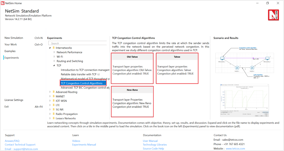
Figure-22: List of scenarios for the example of TCP Congestion Control Algorithms

NetSim UI displays the configuration file corresponding to this experiment as shown below:

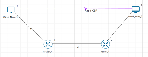
Figure-23: Network set up for studying the TCP Congestion Control Algorithms

Procedure

Old Tahoe

The following set of procedures were done to generate this sample.

Step 1: A network scenario is designed in NetSim GUI comprising of 2 Wired Nodes and 2 Routers in the “Internetworks” Network Library.

Step 2: In the Wired Node 1(Source node), the Congestion Control Algorithm in the Transport layer properties is set to OLD TAHOE.

To configure any properties in the nodes, click on the node, expand the property panel on the right side, and change the properties as described.

Step 3: In the General Properties of In the Wired Node 1(Source node), Wireshark Capture is set to Online.

NOTE: Routers properties are set to default.

Step 4: The link properties are configured as shown in the table below. To set the wired link properties, click on the link, expand the link property panel on the right, and configure the settings as mentioned in the table.

Wired link Properties
Link 2 Properties (Backbone link)
Parameter	Parameter value
Uplink / Downlink Speed (Mbps)	10
Uplink / Downlink BER	0.0000001
Uplink / Downlink Propagation Delay (µs)	50000
Link 1 and 3 Properties
Uplink / Downlink Speed (Mbps)	10
Uplink / Downlink BER	0
Uplink / Downlink Propagation Delay (µs)	100

Table-1: Wired link properties

Step 5: Configure CBR application between Wired node 1 and Wired node 2 by clicking on Set traffic tab from the ribbon on top. To configure application properties, click on created application and set the Packet Size to 1460 Bytes and Inter Arrival Time to 1168 microseconds by keeping the transport layer to TCP.

Step 6: Click on Show/Hide info > Device IP check box in the NetSim GUI to view the network topology along with the IP address.

Step 7: Click on Run simulation. The simulation time is set to 20 seconds.

Tahoe

Step 1: In Wired Node 1 (the source node), the congestion control algorithm is set to TAHOE under the transport layer properties.

Step 2: Run simulation for 20 seconds.

New Reno

Step 1: In Wired Node 1 (the source node), the congestion control algorithm is set to NEW RENO under the transport layer properties.

Step 2: Run simulation for 20 seconds.

Output

We have enabled WireShark Capture in Wired Node 1. The PCAP file is generated during the simulation. From the PCAP file, the congestion window evolution graph can be obtained as follows. In Wireshark, select any data packet with a left click, then, go to Statistics > TCP Stream Graphs > Window Scaling.

The congestion window evolution for Old Tahoe, Tahoe and New Reno congestion control algorithms are presented in Figure-24, Figure-25, and Figure-26, respectively.

Table-2 shows the throughput values of different congestion control algorithms (obtained from the Application Metrics).

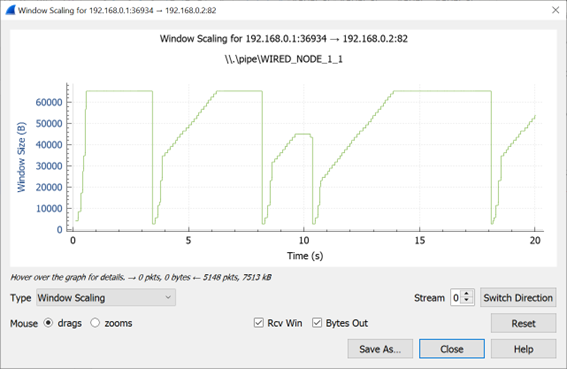
Figure-24: Congestion window evolution with TCP Old Tahoe. We note that Old Tahoe infers packet loss only with timeouts, and updates the slow-start threshold ssthresh and congestion window cwnd as ssthresh = cwnd/2 and cwnd = 1

Figure-25: Congestion window evolution with TCP Tahoe. We note that Tahoe infers packet loss with timeout and triple duplicate acknowledgements, and updates the slow-start threshold ssthresh and congestion window cwnd as ssthresh = cwnd/2 and cwnd = 1

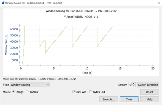
Figure-26: Congestion window evolution with TCP New Reno. We note that New Reno infers packet loss with timeout and triple duplicate acknowledgements and updates the slow-start threshold ssthresh and congestion window cwnd as ssthresh = cwnd/2 and cwnd = ssthresh + 3MSS (in the event of triple duplicate acknowledgements).

Congestion Control Algorithm	Throughput (Mbps)
Old Tahoe	2.98
Tahoe	2.62
New Reno	4.12

Table-2: Long-term average throughput of the different TCP congestion control algorithms

Observations and Inference

We can observe slow start, congestion avoidance, timeout, fast retransmit and recovery phases in the Figure-24, Figure-25, and Figure-26. In Figure-24, we note that Old Tahoe employs timeout, slow-start and congestion avoidance for congestion control. In Figure-25, we note that Tahoe employs fast retransmit, slow-start and congestion avoidance for congestion control. In Figure-26, we note that New Reno employs fast retransmit and recovery, congestion avoidance and slow-start for congestion control.
We note that TCP New Reno reports a higher long term average throughput (in comparison with Old Tahoe and Tahoe, see Table-2) as it employs fast retransmit and recovery to recover from packet losses.

Exercises

1. Impact of Bit Error Rate on TCP Congestion Control Algorithms

Consider the similar experiment, change the BER value \(1 \times 10^{- 7}\), \(2 \times 10^{- 7}\),\(5 \times 10^{- 7}\), \(1 \times 10^{- 6}\) on link 2, simulate it for 500 seconds and compare the performance of TCP Old Tahoe, Tahoe, and New Reno by analyzing the throughput under different error rates. Also, attach the window scaling graph obtained from Wireshark for \(1 \times 10^{- 7}\) case.

2. Performance analysis of TCP congestion control algorithms with varying Maximum Segment Sizes (MSS)

Consider the similar experiment by varying the Maximum Segment Size (MSS) to 500, 700, 900, and 1100 bytes. Simulate the network for 500 seconds and compare the performance of TCP Old Tahoe, Tahoe, and New Reno by analysing the throughput under different segment sizes.

3. Comparative Analysis of TCP Congestion Control Algorithms for Video Application

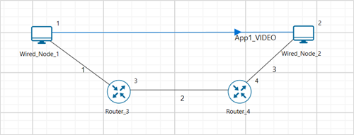
Construct the scenario using 2 Routers and 2 Wired node, set the link properties similar to settings done in experiment, configure a video application with a generation rate of 5 Mbps, set transport protocol to TCP and vary the TCP congestion control algorithm. Tabulate the throughput and jitter values obtained for each case and discuss how each TCP congestion control algorithm affected throughput and jitter. Include window scaling screenshots to support your analysis and highlight any notable differences in the graphs.

Configure the Independent Gaussian model with the following values to generate 5 Mbps of video

\(frames\ per\ second\ (fps)\) = 10

\(pixel\ per\ frame\ (ppf)\) = 961538

\(Mean,\ bits\ per\ pixel\ (bpp\ (µ))\) = 0.52

The generation rate for video application can be calculated by using the formula shown below:

\[Generation\ Rate\ (bits\ per\ second)\ = \ fps\ \times \ ppf\ \times bpp\]

4. Impact of TCP Congestion Control on Video application in Multi-Node Networks

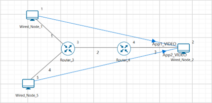
Construct the scenario using 3 wired node and 2 Routers, set the link speed to 20 Mbps, propagation delay and BER to 0, configure a video application with a generation rate of 5 Mbps, set transport protocol to TCP and vary the TCP congestion control algorithm. Tabulate the throughput and jitter values obtained for each case and discuss how each TCP congestion control algorithm affected throughput and jitter.

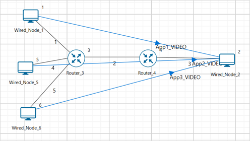
Case a: Increase the transmitter count to 3 (add one more wired node to the existing setup) and create one video application from newly dropped device and increase the bottleneck link capacity to 30 Mbps. Vary the TCP congestion control algorithms and tabulate the throughput and jitter values obtained for each algorithm.

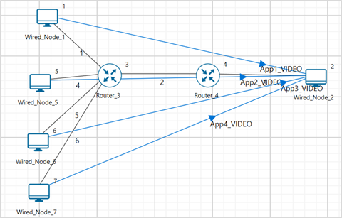
Case b: Increase the transmitter count to 4 (add one more wired node for case a) and create one video application from newly dropped device and increase the bottleneck link capacity to 40 Mbps. Vary the TCP congestion control algorithms and tabulate the throughput and jitter values obtained for each algorithm.

Understand the working of TCP BIC Congestion control algorithm, simulate, and plot the TCP congestion window (Level 2)

Theory

In BIC congestion control is viewed as a searching problem in which the system can give yes/no feedback through packet loss as to whether the current sending rate (or window) is larger than the network capacity. The current minimum window can be estimated as the window size at which the flow does not see any packet loss. If the maximum window size is known, we can apply a binary search technique to set the target window size to the midpoint of the maximum and minimum. As increasing to the target, if it gives any packet loss, the current window can be treated as a new maximum and the reduced window size after the packet loss can be the new minimum. The midpoint between these new values becomes a new target. Since the network incurs loss around the new maximum but did not do so around the new minimum, the target window size must be in the middle of the two values. After reaching the target and if it gives no packet loss, then the current window size becomes a new minimum, and a new target is calculated. This process is repeated with the updated minimum and maximum until the difference between the maximum and the minimum falls below a preset threshold, called the minimum increment (Smin). This technique is called binary search increase.

Additive Increase

To ensure faster convergence and RTT-fairness, binary search increase is combined with an additive increase strategy. When the distance to the midpoint from the current minimum is too large, increasing the window size directly to that midpoint might add too much stress to the network. When the distance from the current window size to the target in binary search increase is larger than a prescribed maximum step, called the maximum increment (Smax) instead of increasing window directly to that midpoint in the next RTT, we increase it by Smax until the distance becomes less than Smax, at which time window increases directly to the target. Thus, after a large window reduction, the strategy initially increases the window linearly, and then increases logarithmically. This combination of binary search increase and additive increase is called as binary increase. Combined with a multiplicative decrease strategy, binary increase becomes close to pure additive increase under large windows. This is because a larger window results in a larger reduction by multiplicative decrease and therefore, a longer additive increase period. When the window size is small, it becomes close to pure binary search increase – a shorter additive increase period.

Slow Start

After the window grows past the current maximum, the maximum is unknown. At this time, binary search sets its maximum to be a default maximum (a large constant) and the current window size to be the minimum. So, the target midpoint can be very far. According to binary increase, if the target midpoint is very large, it increases linearly by the maximum increment. Instead, run a “slow start” strategy to probe for a new maximum up to Smax. So if cwnd is the current window and the maximum increment is Smax, then it increases in each RTT round in steps cwnd+1, cwnd+2, cwnd+4,,, cwnd+Smax. The rationale is that since it is likely to be at the saturation point and also the maximum is unknown, it probes for available bandwidth in a “slow start” until it is safe to increase the window by Smax. After slow start, it switches to binary increase.

Fast Convergence

It can be shown that under a completely synchronized loss model, binary search increase combined with multiplicative decrease converges to a fair share. Suppose there are two flows with different window sizes, but with the same RTT. Since the larger window reduces more in multiplicative decrease (with a fixed factor β), the time to reach the target is longer for a larger window. However, its convergence time can be very long. In binary search increase, it takes log(d)-log(Smin) RTT rounds to reach the maximum window after a window reduction of d. Since the window increases in a log step, the larger window and smaller window can reach back to their respective maxima very fast almost at the same time (although the smaller window flow gets to its maximum slightly faster). Thus, the smaller window flow ends up taking away only a small amount of bandwidth from the larger flow before the next window reduction. To remedy this behaviour, binary search increase is modified as follows. After a window reduction, new maximum and minimum are set. Suppose these values are max_wini and min_wini for flow i (i =1, 2). If the new maximum is less than the previous, this window is in a downward trend. Then, readjust the new maximum to be the same as the new target window (i.e. max_wini = (max_wini-min_wini)/2), and then readjust the target. After that apply the normal binary increase. This strategy is called fast convergence.

Network setup

Open NetSim and click on Experiments> Internetworks> TCP> Advanced TCP BIC Congestion control algorithm then click on the tile in the middle panel to load the example as shown in below Figure-27.

Figure-27: List of scenarios for the example of Advanced TCP BIC Congestion control algorithm

NetSim UI displays the configuration file corresponding to this experiment as shown below Figure-28.

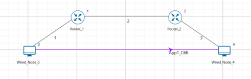
Figure-28: Network set up for studying the Advanced TCP BIC Congestion control algorithm

Procedure

The following set of procedures were done to generate this sample:

Step 1: A network scenario is designed in NetSim GUI comprising of 2 Wired Nodes and 2 Routers in the “Internetworks” Network Library.

Step 2: In the General Properties of Wired Node 3 i.e., Source, Wireshark Capture is set to Online and in the TRANSPORT LAYER Properties, Window Scaling is set as TRUE.

To configure any properties in the nodes, click on the node, expand the property panel on the right side, and change the properties as mentioned in steps.

Step 3: For all the devices, in the TRANSPORT LAYER Properties, Congestion Control Algorithm is set to BIC.

Figure-29: Transport Layer window

Step 4: The Link Properties are set according to the table given below Table-3. To configure link properties, click on link expand the link properties window on right and set as mentioned below.

Link Properties	Wired Link 1	Wired Link 2	Wired Link 3
Uplink Speed (Mbps)	100	20	100
Downlink Speed (Mbps)	100	20	100
Uplink propagation delay (µs)	5	1000	5
Downlink propagation delay (µs)	5	1000	5
Uplink BER	0.00000001	0.00000001	0.00000001
Downlink BER	0.00000001	0.00000001	0.00000001

Table-3: Wired Link Properties

Step 5: Configure applications between two nodes by selecting an application from Set Traffic Tab from ribbon on top. Click on the application flow App1 CBR and expand application property panel on right and start time to 20 seconds, Packet Size set to 1460 Bytes and Inter Arrival Time set to 400 µs.

The Packet Size and Inter Arrival Time parameters are set such that the Generation Rate equals 140 Kbps. Generation Rate can be calculated using the formula:

\[Generation\ Rate\ (Mbps)\ = \ Packet\ Size\ (Bytes)\ *\ 8/Interarrival\ time\ (µs)\]

Step 6: Enable the plots from configure reports tab and click on Run simulation. The simulation time is set to 100 seconds.

Output

Figure-30: Plot of Window Scaling in Wireshark Capture

NOTE: User need to “zoom in” to get the above plot.

Go to the Wireshark Capture window.

Click on data packet i.e. <None>. Go to Statistics -> TCP Stream Graphs -> Window Scaling.

Click on Switch Direction in the window scaling graph window to view the graph.

(For more guidance, refer to section - 8.5 Window Scaling” in user manual)

The graph shown above is a plot of Congestion Window vs Time of BIC for the scenario shown above. Each point on the graph represents the congestion window at the time when the packet is sent. You can observe Binary Search, Additive Increase, Fast Convergence, Slow Start phases in the above graph.