4G LTE

LTE Handover (Level 1)

Handover is a critical process in LTE networks that ensures seamless connectivity and service continuity for mobile users as they move across different cell areas. The goal of handover is to provide the best possible connection by dynamically switching the User Equipment (UE) to the eNodeB (eNB) that offers the best signal and optimal quality of service. This experiment focuses the concepts, algorithms, and procedures involved in LTE handover.

Handover modeling in NetSim

The handover logic in NetSim LTE is based on the Strongest Adjacent Cell Handover Algorithm [1]. The algorithm enables each UE to connect to that eNB which provides the highest signal quality. Therefore, a handover occurs the moment a better eNB i.e., when adjacent cell has offset stronger signal quality is detected. The exact handover algorithm including details of the offset (also known as handover-margin) is explained in the 5G manual.

Use of SNR instead of RSRP

NetSim is a packet-level simulator for simulating the performance of end-to-end applications over various packet transport technologies. NetSim can scale to simulating networks with 100s of UEs, eNBs, routers, switches, etc. In order to achieve a scalable simulation, that can execute in reasonable time on desktop-level computers, many details of the physical layer techniques have been abstracted.

In NetSim LTE, there are no pilots/reference/synchronization signals. The channel matrix H is assumed to be known perfectly and instantaneously at the transmitter and receiver, respectively. Hence there is no RSRP, and all signal power related calculations are done in the SSB channel. Therefore, the hand-over is based on the SNR measured at the source (serving) eNB and the target (neighbouring) eNB. Since the noise power would be the same at s-eNB and t-eNB, in effect the handover is based on received signal level on the SSB.

Control packet exchange

During initial attachment, a UE associates with the eNB from which it sees the highest SNR. The eNB to which a UE is attached is called the serving eNB.
The UE periodically sends the UE MEASUREMENT REPORT to the Serving eNB, which contains the SNRs from all the nearby eNBs. The Serving eNB makes the decision on whether to hand off the UE to a T-eNB (Target-eNB) based on the handover condition

\[SNR_{t - gNB}\ - \ SNR_{s - gNB}\ > \ HOM\]

In NetSim by default the HOM is set to 3 dB.

If the condition is met, the S-eNB issues a HANDOVER REQUEST message to the T-eNB passing necessary information to prepare the handover at the target side.
The T-eNB sends back the HANDOVER REQUEST ACKNOWLEDGE message including a transparent container to be sent to the UE as an RRC message to perform the handover.
The S-eNB generates the RRC (Radio resource control used for signaling transfer) message to perform the handover, i.e., RRC CONNECTION RECONFIGURATION message including the mobility Control Information.
The S-eNB starts forwarding the downlink data packets to the T-eNB for all the data bearers which are being established in the T-eNB during the HANDOVER REQ message processing.
The T-eNB now requests the S-eNB to release the resources. With this, the handover procedure is complete.

Scenario

Open NetSim and Select Experiments > LTE > Handover in 4G then click on the tile in the middle panel to load the example as shown in below screenshot Figure-1.

Figure-1: List of scenarios for the example of LTE Handover

The following network diagram illustrates what the NetSim UI displays when you open the experiment configuration file as shown Figure-2.

Figure-2: Network set up for studying the LTE-Handover

Network Settings

The following set of procedures were done to generate this sample:

Step 1: Environment Grid length: 6000m x 3000m.

Step 2: A network scenario is designed in NetSim GUI comprising of 2 ENBs, 1 EPC, 1UE, 1 Router and 1 server in the “LTE/LTE-A” Network Library.

Step 3: The device positions are set as per the table given below.

	ENB 4	ENB 6	UE 5
X Co-ordinate	1000	4500	1000
Y Co-ordinate	1000	1000	2500

Table-1: Devices positions

Step 4: The eNB properties are set as follows. To configure them, click on the eNB, and in the right panel, expand the window to view all layer properties and set the properties listed below.

Interface (LTE) Properties
CA TYPE	SINGLE BAND
CA Configuration	BAND 42
Component Carrier 1
DL UL Ratio	4:1
Numerology	0
Channel Bandwidth (MHz)	10
PDSCH Configuration
MCS Table	QAM64
CSI Report Configuration
CQI Table	TABLE1
Channel Model
Outdoor Scenario	URBAN MACRO
LOS NLOS Selection	USER DEFINED
LOS Probability	1
Shadow Fading Model	None
Fast Fading Model	No Fading

Table-2: eNB > Interface (LTE) Properties Setting

Similarly, it is set for eNB 6.

Step 5: In the UE 5 device position properties, set Mobility Model as File Based Mobility.

File Based Mobility

In File Based Mobility, users can write their own custom mobility models and define the movement of the mobile users. Create a mobility.csv file for UE’s involved in mobility with each step equal to 0.5 sec with distance 250 m. where the UE moves 2500m away from the eNB 4 towards eNB 6.

The NetSim Mobility File (mobility.csv) format is as follows:

#Time(s)	Device ID	X	Y
0	5	1000	2500
0.5	5	1250	2500
1	5	1500	2500
1.5	5	1750	2500
2	5	2000	2500
2.5	5	2250	2500
3	5	2500	2500
3.5	5	2750	2500
4	5	3000	2500
4.5	5	3250	2500
5	5	3500	2500
5.5	5	3750	2500
6	5	4000	2500
6.5	5	4250	2500
7	5	4500	2500

Table-3: Mobility.csv file

The mobility path for UE 5 can be observed using the mobility viewer as shown below. For more detailed on mobility viewer refer the user manual section 8.6.

Figure-3: Mobility viewer showing the UE 5 mobility path

Step 6: Configure an application between the server 3 (wired node 3) and UE 5 by selecting a CBR application from the Set Traffic tab. The QoS for the CBR application is set to UGS. To configure the QOS, click on the created application and expand the application property in the right, and set the QOS as mentioned.

Step 7: Enable Packet Trace, SNR vs Time plot and Logs in NetSim GUI as shown in below figure. At the end of the simulation, a large .csv file contains all the packet information and is available for the users to perform packet level analysis.

Figure-4: Enabling plots, packet trace and log file.

Step 8: Run the Simulation for 10 Seconds.

Results and Discussion

Handover Signaling

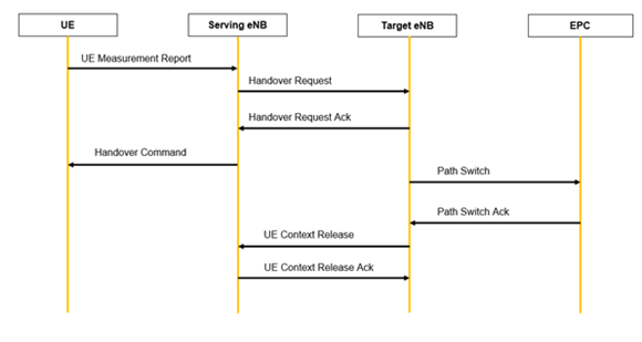
Figure-5: Control packet flow in the LTE handover process

Note:

The Handover Request will be sent from the serving eNB to the target eNB, and the Handover Request Ack will be sent from the target eNB to the serving eNB through the EPC.
The Context Release will be sent from the serving eNB to the target eNB, and the Context Release Ack will be sent from the target eNB to the serving eNB through the EPC.

The packet flow depicted above can be observed from the packet trace.

UE will send the UE (SS/PBCH) MEASUREMENT REPORT every 5 ms to the connected eNB.
The initial UE- eNB connection, eNB will send the RRC MIB packets to the UE every 40 ms and RRC SIB1 every 80 ms.
After the transmission of the RRC MIB and RRC SIB1 packets, the eNB will send RRC_SI packet to the UE.
After reception of RRC SI packet, UE will send RRC Setup Request to the eNB.
On receiving the RRC Setup Request packet, the eNB will acknowledge the request by transmitting RRC Setup packet to the UE.
The UE will send back the RRC Setup Complete packet on the receipt of RRC Setup message.

Figure-6: Packet trace file showing the RRC Initial Association.

As Per the configured file-based mobility, UE 5 moves towards eNB 6.
After 4.5s eNB 4 sends the HANDOVER REQUEST to eNB 6 through EPC 1.
eNB 6 sends back HANDOVER REQUEST ACK to eNB 4 through EPC 1.
After receiving HANDOVER REQUEST ACK from eNB 6, eNB 4 sends the HANDOVER COMMAND to UE 5
After the HANDOVER COMMAND packet is transferred to the UE, the target eNB will send the PATH SWITCH packet to the EPC 1.
When the EPC 1 receives the PATH SWITCH packet, it sends PATH SWICTH ACK packet to the eNB 6.
The target eNB sends CONTEXT RELEASE to source eNB, and the source eNB sends back CONTEXT RELEASE ACK to target eNB. The context release request and ack packets are sent between the source and target eNB via EPC 1.
RRC Reconfiguration will take place between target eNB and UE 5.
The UE 5 will start sending the UE (SS/PBCH) MEASUREMENT REPORT to eNB 6

Figure-7: Packet trace file showing control messages involved during the handover process.

Plot of SNR vs. Time

Figure-8: Plot of the DL SNR over time seen by the UE from the serving cell (eNB 4) and the target cell (eNB 6). The handover process does not commence with Adj. cell SNR is greater than Serving cell SNR but only commences with Adj. cell SNR is greater than Serving cell SNR by the Handover margin (3 dB in this case). The SNR is measured in the SSB channel.

This chart can be obtained in NetSim by enabling the option to plot SNR vs. time prior to the simulation. First, plot the SNR curve for eNB 4 and UE 5 keeping the channel as PDSCH and Layer ID as 1. Then select "Add as new series" and select the gNB/eNB as eNB 6 and UE name as UE 5. Click on plot, and you would then obtain the above "stacked" plot

Time 4.5s when the SNR from eNB 4 is 9.47dB and the SNR from eNB 6 is 15.12dB. This represents the point where Adj cell RSRP is greater than serving cell RSRP by Hand-over margin (HOM) of 3dB.

References

[1] K. Dimou, “Handover within 3GPP LTE: Design Principles and Performance,”Ericsson Research

Impact of Interference in 4G Networks (Level 3)

Objective

In this experiment, we will simulate and study the impact of downlink interference on the signal-to-interference ratio (SINR) in NetSim v14.2. We will study the following aspects.

We consider a handover procedure in a cellular system and analyse the following cases:

The handover of a UE without any interference, with pathloss exponent, \(\eta = 2.5\),
The handover of a UE without any interference, with pathloss exponent \(\eta = 4\),
The handover of a UE with interference, with pathloss exponent \(\eta = 2.5\), and
The handover of a UE with interference, with pathloss exponent \(\eta = 4\).

To understand the effect of path loss exponents with and without interferences on the point of handovers in cellular systems.

In this experiment, we consider the following handover scenario: A UE starts from \(BS_{1}\) and moves in a straight line to \(BS_{2}\). While the UE is attached to \(BS_{1}\) it experiences interference from \(BS_{2}\). Once it gets handed over to \(BS_{2}\ \)the UE experiences interference from \(BS_{1}\). There is always thus only one interferer, and we analyse the SINR as the UE moves a straight line from \(BS_{1}\ \)to \(BS_{2}\).

Figure-9: UE1 is initially attached to BS1. The signal from BS1 is the desired signal while the signal from BS2 is the interfering signal. Post-handover, the desired signal is transmitted from BS2 while signal from BS1 is the interfering signal. We assume omni-directional antennas at both BSs and consider cases with η = 2.5, 4

Introduction

Due to the scarcity of the wireless spectrum, it is not possible in 4G networks to separate concurrent transmissions completely in frequency. Some transmissions will necessarily occur at the same time in the same frequency band, separated only in space, and the signals operating on the same time-frequency resources from many undesired or interfering transmitters are added to the desired transmitter’s signal at a receiver. The main determinants of the interference are,

The network geometry, i.e., the location of the receivers and the transmitters
Base stations’ (or eNBs’) transmit power, and
The path loss model (signal attenuation with distance).

The performance and coverage of a 4G network critically depends on the signal-to-interference-and-noise ratios (SINRs) level at the receivers. This is defined as

\[SINR = \frac{P_{r}}{N_{0}W + I}\]

Where \(P_{r}\) is the received power of the desired signal, \(W\ \)is the bandwidth, \(N_{0}W\) is the thermal noise and \(I\ \)is the received power of interfering signals. In 4G, the modulation and coding scheme (MCS) is computed from the SINR. The higher the SINR, the higher the MCS, and hence the higher the date rate. Interference is therefore an important performance-limiting factor in wireless networks and hence it is crucial to characterize the effect of interference.

Network Simulation Setup

Open NetSim and click on** Experiments > LTE > Impact of Interference in 4G Network**s then click on the tile in the middle panel to load the example as shown in below.

Figure-10: List of scenarios for the example of Impact of Interference in 4G Networks.

ISD = 500m, BAND42, 20 MHz, Urban Macro

In our network scenario, the inter-site distance (ISD) between \(BS_{1}\) and \(BS_{2}\) is 500m. Both base stations (eNB) operate in the 3.4 GHz band, with a bandwidth of 20 MHz. The environment is assumed to be urban with signal attenuation as per the 3G PP Urban Macro pathloss model. Shadow-fading and fast fading are turned off to avoid sources of randomness.

Case 1: No interference in both base stations with η = 2.5

Network Scenario

Figure-11: NetSim Scenario during mobility.

Simulation Parameters

Set grid length as 1600 x 800 from grid setting property panel on the right. This needs to be done before any device is placed on the grid. Place the second eNB 500 meters away from the first eNB

Devices	X	Y
eNB 4	300	600
eNB 5	800	600
UE 6	300	600

Table-4: Device Co-ordinates.

Click on eNB and expand property panel on right and change the properties as mentioned in the below steps. Similarly set the same properties in another eNB.

eNB> Interface LTE
Physical Layer Properties
eNB Height (m)	10
Tx Power (dBm)	40dBm
CA Type	Single Band
CA Configuration	BAND42
Component Carrier 1
DL: UL Ratio	4:1
F Low (MHz)	3400
F High (MHz)	3600
Numerology	0
Channel Bandwidth (MHz)	20MHZ
Antenna
Tx Antenna Count	1
Rx Antenna Count	1
PDSCH and PUSCH Configuration
MCS Table	QAM64
CSI Report Configuration
CQI Table	Table1
Channel Model
Pathloss model	Log distance
Pathloss exponent	2.5
Shadowing model	None
Fast Fading Model	No Fading
Interference Model
Downlink interference model	No interference

Table-5: Values set for different parameters in simulation.

Go to UE properties. In the RAN Interface set physical layer properties in both UEs as shown below.

UE > Interface LTE>Physical Layer
UE Height	1.50
Tx Power	23 dBm
Antenna
Tx Antenna Count	1
Rx Antenna Count	1

Table-6: Properties set for UE

In the General layer, set UE X and Y coordinates as the eNB1’s X and Y coordinates. That is, the initial position of UE must be the position of eNB1.
Set the mobility model as file-based mobility and configure the mobility that UE needs to be travel straight towards to the eNB2. So, configure the mobility file according to the distance that UE needs to travel. For example, in the above scenario, UE needs to travel 500m from eNB1 to eNB2 So, it is travelling straight towards to another eNB since it’s Y coordinate is fixed. Hence, give input in the excel sheet as in Figure-12

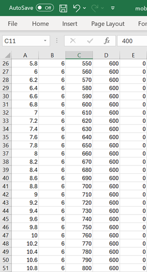
Figure-12: UE Mobility file for 500m

Before clicking on Run, enable “LTENR Radio Measurements Log” as shown in Figure-13

Figure-13: Enabling the Log Options from GUI.

Now, Run the Simulation for 12 s.
After simulation, open LTENR Radio measurement log present under the Log files section in the Results Dashboard as in Figure-14.

Figure-14: ISD 500m simulation result Dashboard.

Figure-15: Inserting Pivot table

Figure-16: Creating Pivot table

Create a pivot table for this log file by clicking the pivot option present at the top of the ribbon under insert section as shown below.
In the pivot table drop ‘gNB/eNB Name’, ‘UE Name’, ‘Channel’ fields under filters area, drop ‘Distance’ in Row area and drop ‘SINR’ in Value area. Set the SINR values to max by clicking on the arrow icon present at the end of the field ->value field setting->max as shown below as shown in Figure-16
Now filter eNB as eNB4, UE name as UE 6, Channel as PDSCH as shown in Figure-16
Copy the values from 0 to 290 along with Row Labels and Max SINR dB header and paste it into another sheet. Similarly filter gNB/eNB name to eNB 5 and copy the row label value along with SINR and paste it into next to the previously created new sheet.
NetSim calculates the distance of a UE from its attached eNB. In the plot that we eventually wish to obtain the X axis has distance from the initial attached eNB which is eNB4. In our experiment, UE6 is initially attached to eNB4 and post-handover it gets attached to eNB5. Since eNB4 to eNB5 distance is 500m, post-handover the distance of UE6 from the initial eNB4 is \(500 - d_{gNB(5)}^{UE(6)}\)i.e., \(d_{gNB(4)}^{UE(6)} = 500 - d_{gNB(5)}^{UE(6)}\).

Copy the Row table and distance to the empty cells after filtering that gNB/eNB Name to eNB5 and UE Name to UE6 as shown in Figure-17

In the adjacent cell calculate the UE 6 distance from eNB 4 as shown below as shown in Figure-18. Observe that it is initially \(d_{gNB(4)}^{UE(6)}\) and post-handover it is \(500 - d_{gNB(5)}^{UE(6)}.\)

Distance between UE6 and eNB4, \(d_{gNB(4)}^{UE(6)}\), along with the SINR value and copy them into new cells.

Filter it from the ascending order/ smallest to largest, copy these values to the paste it below the previously created new sheet as shown in Figure-19

Figure-17: Copying the Distance and SINR values into new cells.

Figure-18: Inserting filter.

Figure-19: Sorting from smallest to largest.

Results

Distance	Max of SNR(dB)
0	69.54
10	69.54
20	64.07
30	60.15
40	57.20
50	54.87
60	52.93
70	51.29
80	49.86
90	48.59
100	47.46
110	46.43
120	45.49
130	44.62
140	43.82
150	43.07
160	42.38
170	41.72
180	41.10
190	40.51
200	39.96
210	39.43
220	38.93
230	38.44
240	37.98
250	37.54
260	37.11
270	36.70
280	36.31
290	35.93

Table-7: Downlink SINR values for eNB 4, with ISD = 500m

Distance	Max of SNR(dB)
290	39.43
300	39.96
310	40.51
320	41.10
330	41.72
340	42.38
350	43.07
360	43.82
370	44.62
380	45.49
390	46.43
400	47.46
410	48.59
420	49.86
430	51.29
440	52.93
450	54.87
460	57.20
470	60.15
480	64.07
490	69.54
500	69.54

Table-8: Downlink SINR results eNB_5, with ISD = 500m

Case 2: No interference in both base stations with η = 4

eNB4 > Interface LTE
Channel Model
Pathloss model	Log distance
Pathloss exponent	4
Interference Model
Downlink Interference	No Interference
eNB5 > Interface LTE
Channel Model
Pathloss model	Log distance
Pathloss exponent	4
Interference Model
Downlink interference	No Interference

Table-9: Properties set for Case 02.

Set the above property values and simulate the scenario for 12 sec. Tabulate the results obtained from LTENR Radio measurement log in the simulation metrics window.

Case 3: UE to Both Base stations is in η = 2.5

eNB 4 > Interface LTE
Channel Model
Pathloss model	LOG DISTANCE
Pathloss exponent	2.5
Interference Model
Downlink Interference	Exact geometric model
eNB 5 > Interface LTE
Channel Model
Pathloss model	Log distance
Pathloss exponent	2.5
Interference Model
Downlink interference	Exact geometric model

Table-10: Properties set for Case 03.

Set the above property values and simulate the scenario for 12 sec. Tabulate the results obtained from LTENR Radio measurement log in the simulation metrics window.

Case 4: UE to Both Base stations with η = 4

eNB 4 > Interface LTE
Channel Model
Pathloss Model	Log distance
Pathloss Exponent	4
Interference Model
Downlink Interference	Exact geometric model
eNB 5 > Interface LTE
Channel Model
Pathloss model	Log distance
Pathloss exponent	4
Interference model
Downlink Interference	Exact geometric model

Table-11: Properties set for Case 04.

Set the above property values and simulate the scenario for 12 sec. Tabulate the results obtained from LTENR Radio measurement log in simulation metrics window.

Results of UE with η = 2.5 and η = 4

Distance	Case #2 DL SINR (dB)	Case #3 DL SINR (dB)	Case #4 DL SINR (dB)
0	52.77	39.52	52.40
10	52.77	39.30	52.37
20	44.01	33.60	43.57
30	37.74	29.45	37.27
40	33.03	26.28	32.52
50	29.29	23.70	28.73
60	26.20	21.52	25.59
70	23.56	19.63	22.90
80	21.27	17.94	20.55
90	19.25	16.42	18.46
100	17.43	15.01	16.57
110	15.79	13.71	14.84
120	14.28	12.49	13.25
130	12.90	11.33	11.76
140	11.62	10.24	10.37
150	10.42	9.18	9.04
160	9.30	8.17	7.78
170	8.25	7.19	6.57
180	7.26	6.24	5.40
190	6.33	5.31	4.27
200	5.44	4.40	3.15
210	4.59	3.50	2.06
220	3.78	2.61	0.97
230	3.01	1.74	-0.11
240	2.27	0.87	-1.20
250	1.57	0.00	-2.30
260	0.89	-0.87	-3.41
270	0.23	-1.74	-4.54
280	-0.40	-2.62	-5.70
280	3.78	-2.62	0.97
290	4.59	-3.50	2.06
290	4.59	3.50	2.06
300	5.44	4.40	3.15
310	6.33	5.31	4.27
320	7.26	6.24	5.40
330	8.25	7.19	6.57
340	9.30	8.17	7.78
350	10.42	9.18	9.04
360	11.62	10.24	10.37
370	12.90	11.33	11.76
380	14.28	12.49	13.25
390	15.79	13.71	14.84
400	17.43	15.01	16.57
410	19.25	16.42	18.46
420	21.27	17.94	20.55
430	23.56	19.63	22.90
440	26.20	21.52	25.59
450	29.29	23.70	28.73
460	33.03	26.28	32.52
470	37.74	29.45	37.27
480	44.01	33.60	43.57
490	52.77	39.30	52.37
500	52.77	39.52	52.40

Table-12: Results for SINR vs. distance for ISD-500m downlink

The red marks indicate the points of handover.

Figure-20: Downlink SINR vs. distance plot for BAND42 for different network configurations.

Discussions

Initially (in case 1), the UE is attached to \(BS_{1}\). In the scenario, the UE moves in a straight line towards \(BS_{2}\) and at 290 m it is handed over to \(BS_{2}.\) Till 290 m the “desired” signal is from \(BS_{1}\) while the “interfering” signal is from \(BS_{2}\). Post-handover there is a reversal; the desired signal is from \(BS_{2}\) while the interfering signal is from \(BS_{1.}\)

Signals from \(BS_{1}\) and from \(BS_{2}\) to the UE undergo pathloss. If the transmit powers at both \(BS\)s are \(P_{t}\) then the \(SINR\ \)works out to be

\[SINR = \frac{P_{t} \times PL(d)}{N_{0} \times W + P_{t} \times PL\left( d_{ISD} - d \right)}\]

Where \(PL(d)\) is the pathloss loss (per the 3GPP pathloss models) at a distance of \(d\). Since the distance between the two \(BS\)s is equal to \(d_{ISD}\), the inter site distance, the UE is at a distance of \((d_{ISD} - d\)) from the interfering \(BS\), and hence the \(PL(d_{ISD} - d)\) term in the denominator. When there is a line-of-sight (LOS) condition with a eNB, the path loss is lower, modelled here by setting the path loss exponent as 2.5. When there is a non-line-of-sight (NLOS) condition with a eNB, the path loss is higher, modelled here by setting the path loss exponent as 4.

With this background, let us look Figure-20

In all cases, we see a constant SINR till 10m because the pathloss equations defined in the standard take effect only from 10m.
SINR. vs distance is plotted for four cases.
- Case #1: UE is in LOS with both BSs, interference is turned off
- Case #2: UE is in NLOS with both BSs, interference is turned off
- Case #3: UE is in LOS with both BSs, with interference turned on
- Case #4: UE is in NLOS with both BSs, with interference turned on
Note: Here, we use the terms LOS for η=2.5, and NLOS for η=4, for simplicity.
In case 1 and case 2, the term \(I\) in \(SINR = \frac{P_{r}}{N_{0}W + I}\) is set to zero. Practically, this means that the two BSs operate in non-overlapping frequency bands. Therefore, \(SINR = SNR = \frac{P_{r}}{N_{0}W}\).\(\ \)We see the SNR dropping as the UE moves away from \(BS_{1}\). At 280/290m, it gets handed over to \(BS_{2}\), and we see the SNR increasing as the UE moves closer to \(BS_{2}\). Why is there a “jump” at the handover point? This is because the standards specify that handover should occur only when target-eNB’s SINR is offset (3 dB) higher than serving-eNB’s SINR. This condition is satisfied at 280m. You are encouraged to think about the question: Why does the standard specify such an offset?
Next, we observe that the NLOS curve (purple) is lower than the LOS curve (blue). This is because NLOS pathloss is higher than the LOS pathloss.
In Cases 3, and 4, the observations are similar to the above, but they are lower than their respective counterparts in cases 1 and 2, due to additional interferences which degrade the SINR further. Further, we notice that the two curves of cases 2 and 4 are very close to each other. Why?

Open the log files for these cases and observe the following: The pathloss is more pronounced in these cases, and the interference also decays faster than the case (3) case. Hence, the effect of interference is not very pronounced, leading to almost similar performance.

Optional Exercise: Check whether the gap between the two curves increases by increasing eNB transmit powers (i.e., increasing the interference power).

Understanding the points of handoff

For the sake of exposition, we investigate the point of hand-off for case #1 and case #2 where the interferences are assumed to be absent from the base-stations. This therefore represents a noise limited regime, or a scenario where the two BSs use non-overlapping frequency bands. In such a scenario, as the UE moves from BS1 towards BS2, the SNR from BS1 decreases, while the SNR from BS2 increases. The point where the SNR from BS2 is 3 dB higher than that from BS1 determines the point of handoff. But we observe that between the cases with path loss exponents of 2.5 and 4, the points of handovers are different! Why? Read the discussion below.

Further Discussion

For the sake of generality, we discuss the effect of path loss exponent on handover in a general setting independent of the values obtained in the experiment. Consider the scenario:

Figure-21: Illustration of different handover points in LOS/NLOS cases.

Case A: Noise limited scenario

Let a UE move from base station A towards base station B with inter site distance = 1 km as shown in Figure-21. Consider for the moment that we are in a noise-limited regime, where the interferences are assumed to be absent from the base-stations. In such a scenario, as the UE moves from BS A towards BS B, the SNR seen by the UE from BS A decreases, while the SNR seen from BS B increases. For example, let the path loss exponent be set to 1 (ƞ=1), then solid blue curve represents the received SNR as a function of distance seen from BS A, while solid purple curve represents the received SNR as a function of distance seen from BS B. Further, assume that \(\mathrm{\Delta}_{HO}\) is the “handoff threshold” or “handover margin”, i.e., the required SNR difference between the base stations in order to perform a handoff from BS A to BS B. Let the distance at this point be d₀. This point is indicated by point Y in the above plot.

However, when the path loss exponent increases to 2, i.e., ƞ=2, the received SNR from both the BSs changes and the corresponding curves are shown in the above figure using dashed lines. Clearly, due to the differing slopes in the SNR curves at different values of ƞ, the point at which the handoff occurs is different (in fact it occurs earlier than the former case) and this point is indicated by X.

Conclusion: The point of handoff is different for environments with different pathloss exponents for a given handoff threshold.

Remarks: Observe from the figure that, as we increase the path loss from 1 to 2, the point of handoff occurs at d = 1.7 Km and d = 1.76 Km, respectively. This difference is more pronounced when the pathloss difference increases.

Case B: Interference limited scenario

In this case, a similar plot (like above) can be used for handoff analysis, except that y-axis will now have the SINR instead of SNR. It is an exercise for the reader to understand and explain the impact of interference on the handover points in the LOS/NLOS cases.

References

[1] M. Haenggi and R. K. Ganti, “Interference in Large Wireless Networks,” 2009.

Understanding the Impact of MAC Scheduling algorithms on throughput, in a multi-UE scenario (Level 2)

Introduction

Base stations (eNBs) generally deal with multiple mobile stations UEs, some of which require larger bandwidths than others and some of which have better connections (signal quality) than others. In ideal circumstances the base station has plenty of resources (e.g., bandwidth) and each UE gets the resources it needs. However, usually resources are limited, and the base station needs some way of fairly allocating the resources between the UEs.

Consider the downlink of a single eNB 4G cellular system. Several UEs are receiving data from ongoing transfers, for example, TCP controlled file downloads. Assuming that the bottleneck on the transfer path for these connections is this eNB to UE wireless access, the downlink per-UE queues in the eNB will be nonempty. At the beginning of each downlink slot (TTI) the eNB scheduler has to decide which of the UEs’ waiting data to transmit in that slot.

At each eNB the MAC scheduler decides the PRB allocation, per carrier, per TTI (slot), in the PDSCH (DL) and in the PUSCH (UL). Control packets such as the buffer status report (BSR) and UL assignment, are assumed to be sent out of band. The resources for transmission of these control packets are part of Overhead as defined in 3.9.21 5G manual.

Round Robin Scheduler

It divides the available PRBs among the active flows, i.e., those logical channels which have a non-empty RLC queue. The MCS for each user is calculated according to the received CQIs.

Proportional Fair Scheduler

For data transfers, an important performance measure is long term throughput in bits/second, say, \(T_{i}\),\(1 \leq i \leq n\), where \(n\) is the number of UEs. One approach to designing a scheduler is to evaluate the goodness of the throughput vector \(\left( T_{1},\ \ldots,\ T_{n} \right)\) by a network utility, which is the sum of individual user utilities. The utility (or, usefulness) of a throughput \(T\), to a user, increases with increasing throughput, but for large throughputs, increasing throughput further gives diminishing increase in usefulness. This property is modeled as a nondecreasing concave function of throughput. A common measure of utility is the log function, i.e., for the throughput vector \(\left( T_{1},\ \ldots,\ T_{n} \right)\), the utility of throughput \(T_{i}\) to user \(i\) is measured as \(\ln T_{i}\). The network utility is, then, given as

\[\sum_{i = 1}^{n}{\ln T_{i}}\]

A Proportional Fair (PF) scheduler works by scheduling users in slots so that the utility of their long-term throughputs is maximized. In the 4G setting, the scheduling decisions at the beginning of a TTI are based on the physical rates that each UE can get in each Resource Block (RB). If we are given statistical models of these rates, then a nonlinear optimization problem can be formulated and solved to obtain the schedule. This is not a practical approach, however, and a learning algorithm is desired, which, based on slot-by-slot CSI measurements, takes scheduling decisions, which lead to PF optimal throughputs.

The Proportional Fair Scheduler is such a learning scheduler, that uses the throughputs that users are expected to get in the next slot, and the average throughputs they have each obtained up to this slot, to decide which UEs to schedule in the next slot. The practical PF scheme, described below, is based on information such as a presently available data rate for each user in each RB in the next slot (obtained by CSI measurements), and an average data rate over an immediately prior predetermined interval for each user.

Implementation

Since NetSim uses a flat fading model, in each slot, each UE achieves the same MCS in every RB in that slot. In other words, different UEs achieve, possibly, different MCSs, but a single UE has the same MCS across all RBs in a slot. Under this assumption, it is optimal to schedule the same UE in every RB in that slot. Since the channel condition can stochastically vary from slot to slot, the MCSs that the UEs achieve will vary from slot to slot. Under this assumption, the following algorithm is Proportional Fair optimal.

Let \(i,j\) denote generic users and let \(t\) be the slot index. A resource block index \(k\) is required given the flat fading assumption. Let \(M_{i}(t)\) be the MCS seen by user \(i\) at time (slot) \(t\). The channel CQI (derived from the data channel SINR) is used by the adaptive modulation and coding (AMC) module to determine the MCS. We denote by \(S(M,B)\) the TB size in bits for a given MCS, \(M\), and a given number of physical resource blocks (PRBs), \(B\). The achievable rate \(R_{i}(t)\) in bit/s for user \(i\) in slot \(t\) is defined as

\[R_{i}(t) = \frac{S\left( M_{i}\ (t),\ 1 \right)}{\tau}\]

where \(\tau\) is the TTI, i.e., 1 slot duration. At the start of each slot \(t\), the user index \(i^{*}(t)\) - selected by the scheduler - to which required PRBs (per that user’s demand) is assigned at time \(t\) is determined as

\[i^{*}(t) = \underset{j = 1,\ \ldots,N}{argmax}\left( \frac{R_{j}(t)}{T_{j}(t)} \right)\]

This selection is carried out by the scheduler till all PRBs in slot \(t\) are allocated. In the above expression, \(T_{j}(t)\) is the past throughput performance perceived by the user \(j\), and is defined as

\[T_{j}(t) = \left( 1 - \frac{1}{\alpha} \right)T_{j}(t - 1) + \frac{1}{\alpha}\ {\widehat{T}}_{j}(t)\]

Where \(\alpha\) is the time constant (in units of slots) of the exponential moving average. NetSim uses \(\alpha = 50\), and \({\widehat{T}}_{j}(t)\) is the actual throughput achieved by the user \(i\) in the subframe \(t\). If \({\widehat{B}}_{j}(t)\) is the number of PRBs allocated to user \(j\), we finally get

\[{\widehat{T}}_{j}(t) = \frac{{S(M}_{j}(t),\ {\widehat{B}}_{j}(t))\ }{\tau}\]

The value of \(\alpha\) can be changed by the user by editing the NetSim’s source code; it cannot be changed via the GUI. The PF scheduler thus selects a user having the maximum among values obtained by dividing a present possible data rate by an average data rate during a predetermined interval at every scheduling time point.

Max Throughput Scheduler

The Max Throughput (MT) scheduler aims to maximize the overall throughput of the Base station (eNB). It allocates each PRBs to the user that can achieve the maximum achievable rate in the current TTI. The highest achievable rate is calculated by wideband MCS, that is derived from the CQI which in-turn is computed from the SINR. The scheduler allocates the required PRBs to this UE in the current TTI (slot). The calculation of achievable rate is similar to what is explained in PF scheduler.

We denote \(S(M,\ B)\) as the TB size in bits for a given MCS, \(M\), and a given number of physical resource blocks (PRBs), \(B\). The achievable rate \(R_{i}(t)\) in bit/s for user \(i\) at slot \(t\) is defined as

\[R_{i}(t) = \frac{S\left( M_{i}\ (t),\ 1 \right)}{\tau}\]

where \(\tau\) is the TTI i.e., 1 slot duration. At the start of each slot \(t\), the user index \(i^{*}(t)\) - selected by the scheduler - to which required PRBs (per that user’s demand) is assigned at time \(t\) is determined as

\[i^{*}(t) = \underset{j = 1,\ \ldots,N}{argmax}\left( R_{j}(t) \right)\]

While MT can maximize cell throughput, it cannot provide fairness to the UEs that experience poor channel condition.

When there are several UEs having the same achievable rate, NetSim implements RR scheduling amongst these UEs that have the same achievable rate.

Network simulation setup

Open NetSim and click on Experiments> LTE > Scheduling in LTE > Multi UE throughput with UEs at different distances and channel is not time varying then click on the tile in the middle panel to load the example as shown in below.

Figure-22: List of samples under scheduling in LTE for Multi UE throughput with UEs at different distances and channel is not time varying.

Part I: Multi UE throughput with UEs at different distances and channel is not time varying

In this example we understand how the scheduling algorithm affects the UDP download throughput of a multi-user (UE) system where the UEs are at different distances from the eNB.

The following network diagram illustrates what the NetSim UI displays when you open this example configuration file.

Figure-23: Network set up for studying the Scheduling example.

Configuring the scheduling algorithm, and parameter settings in example config files

Set grid length as 12000m× 6000m from grid setting property panel on the right. This needs to be done before any device is placed on the grid.
Set distance as follows.

eNB 4 to UE 5 = 1500m

eNB 4 to UE 6 = 2000m, and

eNB 4 to UE 7 = 2500m

Click on eNB, expand the properties panel on right and go to Interface (LTE), set the following properties as shown below table. In the first sample the scheduling type is set to Round Robin, in the second to Proportional fair, and in the third to Max throughput.

Properties
Data Link Layer Properties
Scheduling Type	Varies: Proportional Fair, Max throughput, Round Robin
Physical Layer Properties
CA Type	Single band
CA Configuration	BAND33
CC1
Numerology	0
Channel Bandwidth	20 MHz
Outdoor Scenario	Urban macro
Channel Model Properties
LOS NLOS Selection	User defined
LOS Probability	1
Pathloss model	3GPPTR38.901-7.4.1
Shadow Fading Model	None
Fast Fading Model	No Fading

Table-13: eNB >Interface (LTE) >Data Link layer and Physical Layer properties

Set Tx Antenna Count as 1 and Rx Antenna Count as 1 in eNB properties.
Set Tx Antenna Count as 1 and Rx Antenna Count as 1 in all the UEs.
Configure the application from the Set Traffic tab in the ribbon at the top. Expand the application properties panel on the right and set the following properties as shown below table.

Application Properties
	Application 1	Application 2	Application 3
Application Type	CBR	CBR	CBR
Source ID	3	3	3
Destination ID	5	6	7
QoS	UGS	UGS	UGS
Transport Protocol	UDP	UDP	UDP
Packet Size	1460Bytes	1460Bytes	1460Bytes
Inter-arrival time	116.8μs	116.8μs	116.8μs
Start Time	0s	0s	0s

Table-14: Application properties

Run Simulation for 1.5s and note down throughput value in the results window in each sample. Recall that each sample has a different scheduling algorithm configured.

Results and discussions

The results with all the three UEs simultaneously downloading data is as given below.

Throughput (Mbps)
Scheduling	Application 1	Application 2	Application 3	Aggregate
Round Robin	17.77	11.85	8.29	37.92
Proportional Fair	17.77	11.86	8.28	37.92
Max Throughput	53.33	0	0	53.33

Table-15: UDP download throughputs for different scheduling algorithms when all three 3 UEs simultaneously downloading data

Next, consider a scenario with only one of the UEs seeing DL traffic (we don’t provide inbuilt configuration file for this, and since it is a simple exercise for a user) First, run for the UE at 1500m, then for UE at 2000m and finally for UE at 2500m. This gives the maximum achievable throughput per node since the eNB resources (bandwidth) is not shared between 3 UEs and is fully dedicated to just one UE. The results are below

Distance from eNB (m)	Application ID	Throughput (Mbps)	Remarks
1500	1	53.33	UE 1 alone has full buffer DL traffic
2000	2	35.55	UE 2 alone has full buffer DL traffic
2500	3	24.88	UE 3 alone has full buffer DL traffic

Table-16: UE throughputs if they were run standalone (without the other UEs downloading data)

The PHY rate is decided by the received SNR. Therefore, a UE closer to the eNB will get a higher date rate than a UE further away. In this example the distances from the eNB are such that UE12 Distance > UE11 Distance > UE10 Distance.

In Round Robin PRBs are allocated equally among all three nodes. However, throughputs are in the order UE10 Distance > UE11 Distance > UE12 Distance because of their distances from the eNB. The individual throughputs seen by each of the UEs is exactly \(\frac{1}{3}\) of the throughput as shown in Table-16.The PF scheduler results will match that of the RR scheduler since the channel is not time varying. In Max throughput scheduling the PRBs are allocated such that the system gets the maximum download throughput. The nearest UE will get all the resources and its throughput will be 3 times the throughput of the UE which got the max throughout in RR.

Part II: Multi UEs at different distances with a time varying channel

Figure-24: List of samples under scheduling in LTE for Multi UEs at different distances with a time varying channel.

Configuring the scheduling algorithm, and parameter settings will remain the same for the case below

eNB properties are as follows

Click on eNB, expand the properties panel on right and go to Interface (LTE), set the following properties as shown below. In the first sample the scheduling type is set to Round Robin, in the second to Proportional fair, and in the third to Max throughput.

Properties
Data Link Layer Properties
Scheduling Type	Varies: Proportional Fair, Max throughput, Round Robin
Physical Layer Properties
CA Type	Single band
CA Configuration	BAND33
CC1
Numerology	0
Channel Bandwidth	20 MHz
Channel model properties
Outdoor Scenario	Urban macro
LOS NLOS Selection	User defined
LOS Probability	1
Pathloss model	3GPPTR38.901-7.4.1
Shadow Fading Model	None
Fast Fading Model	Rayleigh
Channel Rank/MIMO Layers	Max Rank
MIMO Beamforming Model	Eigne BF

Table-17: eNB >Interface (LTE) >Data Link and Physical layer properties

Run Simulation for 1.5s and note down throughput value in the results window in each sample.

Results and discussions

The results with all the three UEs simultaneously downloading data are as given below

Throughput (Mbps)
Scheduling	Application 1	Application 2	Application 3	Aggregate
Round Robin	13.51	10.62	7.02	31.15
Proportional Fair	16.99	13.41	9.23	39.63
Max Throughput	32.31	9.82	2.49	44.62

Table-18: UDP download throughputs for different scheduling algorithms when all three 3 UEs simultaneously downloading data with time varying channel.

A difference in the performance of the RR and PF schedulers can be seen when the channel is time varying (of the order of the coherence time which is 10ms). To induce time varying randomness in the channel we enable fading and beamforming. Thus, after every 10ms, NetSim draws an i.e. fading random variable, as the additional loss. Under these conditions, the RR scheduler would allot resources to the UEs in a round robin fashion, whereas the PF scheduler would give preference to the UE which sees the best channel (highest SINR). The reason why the RR scheduler yields lower throughputs than the PF scheduler is that the RR scheduler is not “opportunistic,” i.e., it does not take advantage of the knowledge that a UE has a good channel in the next slot and continues to serve the UEs cyclically. The results are shown in Table-18, observe how this is different from Table-15 where the channel is not time varying.