5G NR
MIMO Beamforming in 5G: A start with MISO and SIMO
Objective: Consider 5G communication between a gNB and single UE, over a fading channel. Setup the simplest MIMO cases, namely MISO and SIMO, and investigate the questions:
How does beamforming gain vary with antenna count?
How does throughput vary with antenna count?
Theory: Multiple input multiple output (MIMO) is a method for increasing the capacity of the wireless channel using multiple transmitting and receiving antennas. Multiple antennas exploit the spatial dimension, i.e., multiple paths from transmitter to receiver, under suitable spacing within the antenna array, on each side, and channel scattering conditions.
Consider a \(N_{t} \times N_{r}\) MIMO system where \(N_{t}\) is the number of transmit antennas and \(N_{r}\) is the number of receive antennas. The simplest MIMO instantiations are when:
\(N_{r} = 1\), a special case where the MIMO system reduces to a Multiple Input Single Output (MISO) channel, and
Reciprocally when, \(N_{t} = 1\), a special case where the MIMO system simplifies into a Single Input Multiple Output (SIMO) channel.
In both SIMO and MISO, the number of layers (i.e., spatial streams with independent data) is \(\min{(N_{t},\ N_{r})},\ \)which equals 1.

Figure-1: Top) Single transmit antenna and multiple receive antennas. Bottom) Multiple Transmit and single receive antenna. In both, \(h_{ij}\) represents the channel between the \(i^{\text{th}}\) receive antenna and the \(j^{\text{th}}\) transmit antenna.
SIMO: SIMO occurs where the transmitter has a single antenna, and the receiver has multiple antennas. The signal received on multiple antennas is combined in order to maximize an appropriate metric. For example, when the goal is to maximize the received SNR, under additive white Gaussian noise, the optimal receiver is called maximal ratio combining. In the case of fading channels (e.g., with Rayleigh fading, explained in the next section), the channels between the transmitter and the different receive antennas is modelled as independent and identically distributed with unit variance entries; this is shown in Figure-1 above. In this case, maximal ratio combining uses the channel coefficients as the weights to combine the signals, and in turn, this provides receive diversity gain. The average SNR at the receiver improves by \(10\ \log_{10}(N_{r})\). However, the improvement in SNR is not exactly the same for every channel instantiation since the channel is random. In this experiment, we will quantify the improvement in the data rate as we vary \(N_{r\ }.\)
MISO: The phase of the signal from each of the transmit antennas is adjusted so that they add constructively at the receiver, yielding an \(N_{t}\ \)fold power gain on average. As with SIMO, the instantaneous SNR gain, however, will differ from \(N_{t}\) since the channel is random. So, the question is, given a choice between having multiple antennas at either the transmitter or the receiver, which option yields better improvement in the throughput? Or will they be the same? Note that, with a single-antenna receiver, only one data stream is transmitted, and therefore multiple antennas offer only a diversity gain, but not a multiplexing gain. Now, practically speaking, is it better to have multiple antennas at the base station or at the user? In terms of antenna placement, there is more space to install antennas at the base station. In addition, the signal processing capability of the base station is much higher than that of a mobile phone. Thus, multiple antennas at the base station are easier to implement than multiple antennas at the mobile phone.
The Rayleigh Fading Channel: For a transmitter (gNB) with \(N_{t}\) antennas and a receiver with \(N_{r}\) antennas, the \(N_{r} \times N_{t}\) baseband channel gain matrix (to model fading between every transmit-receive antenna pair) has complex Gaussian distributed elements. The standard model (under the assumption of Rayleigh fading) is that the complex elements are statistically independent across antennas, and each element is a circularly symmetric complex Gaussian distributed with zero mean and unit variance. We denote this matrix by \(H.\)
For the channel matrix H defined as above, consider the complex Wishart Matrix defined as follows:
\(W = H\ H^{\dagger}\ \ \ \ \ \ r < t\),
\(W = \ H^{\dagger}H\) \(r \geq t\)
Therefore, letting\(\ m = \min{(r,t),\ }\ \) \(W\ \)is an \(m \times m\ \) nonnegative definite matrix, with eigenvalues \(\lambda_{1} \geq \lambda_{2} \geq \lambda_{3} \geq \cdots \geq \lambda_{L} > 0 = \ \lambda_{L + 1} = \cdots = \ \lambda_{m}.\ \)It is these eigenvalues that determine the gains in the parallel SISO models that arise from eigen-beamforming at the transmitter and receiver.
NetSim permits the user to enable or disable a stochastic fading model. Fading is modelled by the elements of \(H\ \)being time varying, with some coherence time. Such time variation results in the eigenvalues of \(W\) also to vary over time. NetSim models such time variation by letting the user define a coherence time during which the eigenvalues are kept fixed. For each \((r,t)\) value, NetSim maintains a list of samples of eigenvalues for the corresponding Wishart matrix.
Network Simulation set up
Open NetSim and click on Experiments > 5G NR > MIMO Beamforming in 5G > Multiple input single output (MISO) in 5G then click on the tile in the middle panel to load the example as shown in below.

Figure-2: List of samples under MIMO Beamforming in 5G for MISO.
Network Scenario:
NetSim UI would display the network topology shown in the screenshot below when you open the example configuration file.

Figure-3: Network topology in this experiment.
Part 1- MISO. Network Configuration
The following parameters were configured in the network setup:
The gNB- Interface 5G RAN were set with the following properties:
gNB- Interface 5G RAN Parameters |
|
|---|---|
gNB Height |
10m |
Tx Power |
40 dBm |
Duplex Mode |
TDD |
CA Type |
Single band |
CA Configuration |
n78 |
Component Carrier 1 |
|
DL: UL Ratio |
4:1 |
Numerology |
0 |
Channel Bandwidth (MHz) |
10 |
Antenna |
|
Tx Antenna Count |
Varied from 1 to 128 |
Rx Antenna Count |
1 |
PDSCH and PUSCH Configuration |
|
MCS Table |
QAM64 |
CSI Report Configuration |
|
CQI Table |
Table1 |
Channel Model |
|
Pathloss model |
3GPPTR38.901-7.4.1 |
Outdoor Scenario |
Urban macro |
LOS NLOS Selection |
User defined |
LOS Probability |
0 (NLOS) |
Shadow Fading Model |
None |
Fast Fading Model |
Rayleigh |
Channel rank/MIMO Layers |
Max Rank |
MIMO Beamforming Model |
Eigen BF |
Coherence Time (ms) |
10 |
Additional Loss Model |
None |
Table-1: gNB properties
The UE properties were configured with the following parameters:
UE Interface 5G RAN |
|
|---|---|
Physical Layer Properties |
|
UE Height |
1.5m |
Tx Power |
23 dBm |
Antenna |
|
Tx Antenna Count |
1 |
Rx Antenna Count |
1 |
Table-2: UE properties
The wired link speed was set to 10 Gbps and the Uplink and Downlink BER were set to 0 in the wired links.
A downlink CBR application was configured from wired node to UE with Transport protocol as UDP and Packet Size of 1460 Bytes and Inter Arrival time of 179.69 µs and the Start Time was set to 1s.
Click on the Configure report tabs and then click on the Plots icon in the toolbar to enable LTENR Radio measurements under Network Logs and Beamforming Gain vs. Time in LTENR Radio Measurements as shown in Figure-4 and Figure-5.

Figure-4: Enabling the LTENR Radio measurement log.

Figure-5: Enabling Beamforming Gain vs Time plot.
Run simulation for 10s, note down the Application Throughput obtained from the Application Metrics table in the NetSim Results dashboard. Similarly, observe the average Beamforming Gain in dB obtained for the DL application from the generated NetSim plot.
Part 2- SIMO. Network Configuration:

Figure-6: List of experiments under MIMO Beamforming in 5G for SIMO
Set all the properties same as part 1- MISO.
Set the Tx Antenna count in 5G RAN interface of gNB to 1.
Vary the Rx Antenna count in 5G RAN interface of UE from 1 to 16.
Run simulation for 10s.
After the simulation, note down the Application Throughput obtained from the Application Metrics table in the NetSim Results dashboard. Similarly, observe the average Beamforming Gain in dB obtained for the DL application from the generated NetSim plot.
Simulation Output:
Steps to calculate the Throughput, Beamforming Gain, SNR, Pathloss and CQI Index:
After the simulation, open NetSim Result dashboard and note down the throughput from the Application Metrics Table as shown below:

Figure-7: NetSim Results window showing Application Throughput obtained after the simulation.
In the results window, click on the Logs option in the left panel and select LTENR Radio Measurements Log.csv file.

Figure-8: NetSim Results window showing access to log file generated.
This will open the csv file which logs the parameters beamforming gain, CQI and MCS Indexes, Pathloss etc. over time as shown below.

Figure-9: LTENR Radio measurement log file generated post simulation.
Filter the Channel to only PDSCH and click on ok since we have considered a DL application from server to UE.

Figure-10: LTENR Radio measurement log file showing the filtering process of PDSCH/PUSCH column
Now select the Beamforming Gain column and note down the average Beamforming Gain in dB per layer.

Figure-11: LTENR Radio measurement log file showing average Beamforming Gain obtained.
Select the Pathloss column and note down the average pathloss value obtained.

Figure-12: LTENR Radio measurement log file showing average Pathloss obtained.
In the same way, select the SNR column and note down the average SNR obtained.

Figure-13: LTENR Radio measurement log file showing average SNR obtained
Similarly, calculate the average CQI Index and MCS Index.

Figure-14: LTENR Radio measurement log file showing average CQI Index obtained.

Figure-15: LTENR Radio measurement log file showing average MCS Index obtained.
Results
MISO: Varying Tx Antenna count in the gNB and 1 Rx Antenna in the UE
gNB_Tx Antenna Count |
UE_Rx Antenna Count |
Throughput (Mbps) |
Average Beam Forming Gain (dB). Number of layers = 1 |
Upper bound for beam forming gain (dB) |
Pathloss (dB) |
Average SNR (dB) |
Average CQI Index |
Average MCS Index |
|---|---|---|---|---|---|---|---|---|
1 |
1 |
0.43 |
-2.70 |
0 |
153.54 |
-12.42 |
0.59 |
0.15 |
2 |
1 |
1.00 |
1.67 |
3.01 |
153.54 |
-8.04 |
1.44 |
0.55 |
4 |
1 |
2.04 |
5.40 |
6.02 |
153.54 |
-4.31 |
2.88 |
2.03 |
8 |
1 |
3.78 |
8.70 |
9.03 |
153.54 |
-1.01 |
4.42 |
4.85 |
16 |
1 |
6.56 |
11.90 |
12.04 |
153.54 |
2.18 |
6.25 |
8.90 |
32 |
1 |
10.27 |
14.97 |
15.05 |
153.54 |
5.25 |
7.93 |
12.87 |
64 |
1 |
14.80 |
18.02 |
18.06 |
153.54 |
8.29 |
9.94 |
17.81 |
128 |
1 |
19.38 |
21.06 |
21.07 |
153.54 |
11.34 |
11.41 |
20.83 |
Table-3: NetSim simulation output showing Throughput, Average beamforming gain and the upper bound (from Jensen’s inequality) on the beamforming gain for a \(N_t \times 1\) channel.
SIMO: Varying Rx Antenna count in the UE and 1 Tx Antenna in the gNB
gNB_Tx Antenna Count |
UE_Rx Antenna Count |
Throughput (Mbps) |
Average Beam Forming Gain (dB). |
Upper bound for beam forming gain (dB) |
Pathloss (dB) |
Average SNR (dB) |
Average CQI Index |
Average MCS Index |
|---|---|---|---|---|---|---|---|---|
1 |
1 |
0.43 |
-2.70 |
0 |
153.54 |
-12.42 |
0.59 |
0.15 |
1 |
2 |
1.00 |
1.67 |
3.01 |
153.54 |
-8.04 |
1.44 |
0.55 |
1 |
4 |
2.04 |
5.40 |
6.02 |
153.54 |
-4.31 |
2.88 |
2.03 |
1 |
8 |
3.78 |
8.70 |
9.03 |
153.54 |
-1.01 |
4.42 |
4.85 |
1 |
16 |
6.56 |
11.90 |
12.04 |
153.54 |
2.18 |
6.25 |
8.90 |
Table-4: NetSim simulation output showing Throughput, Average beamforming gain and the upper bound (from Jensen’s inequality) on the beamforming gain for a \(1 \times N_r\) MIMO channel. \(N_r\) is limited to 16 since this is the maximum antenna count supported in UEs in NetSim.
Beamforming Gain Plot
Open the beamforming gain plot from the simulation result window and disable the Accelerate Plotting and filter the channel to PDSCH and layer ID to 1 and click on plot and observe as following.

Figure-16: NetSim Beamforming Gain vs time plot showing variation in beamforming gain (dB) over the course of simulation. The beamforming gain changes every “coherence time”.
Discussion
From the tabulated results, we observe:
An increase in beamforming gains as
\(N_{t}\) increases in the MISO case, and as
\(N_{r}\ \)increases in the SIMO case.
The beamforming gain when \(N_{t}\) varies (with \(N_{r}\) fixed) is precisely the same as when \(N_{r}\) varies (with \(N_{t}\ \)fixed).
Next, we turn to the question a network engineer would be interested in: how does beamforming impact throughput? While link level simulators may perform the beamforming computations and provide the SNR at a link level, the power of a “system” level simulator like NetSim lies in its ability to compute the impact of link level factors (such as beamforming) on the system (or network). These computations are explained in an earlier experiment.
Since the distance between the gNB and UE is fixed, the common pathloss for all Tx-Rx antenna pairs is the same. This common pathloss value is factored (or “pulled out”) from the individual \(N_{t}\) - \(N_{r}\) path loss calculations. With this factorization done, the only parameter affecting SNR is the channel fading, the effect of which shows up in the output as beamforming gain. Quite simply as the (average) beamforming gain increases, the (average) SNR proportionally increases. Notice that every time the antenna count is doubled the SNR increases by \(\approx \ \)3 dB (which matches intuition). An increase in SNR improves the channel quality (the CQI), and thereby a higher modulation and coding scheme (MCS) is chosen for data transmission.
Remark. Note that these are “average” arguments: in practice, since the fading coefficients are random, one does not obtain a 3 dB improvement by doubling the number of antennas for every channel instantiation. Consequently, the improvement in the spectral efficiency (the reader should study and understand this terminology) is not exactly 1 bit/s/Hz on average. In other words, there is a difference between using the average SNR for computing the data rate versus computing the average data rate by averaging the rate obtained across different channel instantiations. The reader should carry out experiments with different values of \(N_{t}\) and observe the variation in the rate obtained and understand this phenomenon.
Continuing from before the remark, from the MCS the PHY rate is calculated via the procedure for TBS determination per the 3GPP standard. Without getting into the details of these computations, the simplistic inference is that higher MCS leads to higher throughputs.
And finally, the underlying mathematics. The beamforming gains (in linear scale) are the Eigen values of the Wishart matrix. In the MISO and SIMO cases the Wishart matrix has just one element, which itself is the eigenvalue, i.e., the beamforming gain is
Where \(h_{i}\) are the elements of the Wishart matrix, and \(N = N_{t}\) or \(N = N_{r},\) as the case may be. Since \(\mathbb{E}\left| h_{i} \right|^{2} = 1,\)
Since the standard deviation of an exponentially distributed random variable is the square of its mean, and since the \(\left| h_{i} \right|\ 1 \leq i \leq N,\ \)are independent,
However, the beamforming gains output by NetSim are in dB (log) scale. How does one analytically verify its correctness? The answer lies in Jensen’s inequality. Since the log function is concave, Jensen’s inequality leads to
Here \(\lambda\) is the eigen value of the Wishart matrix, and \(10\log_{10}\lambda\) is the beamforming gain in dB scale. Therefore, the beamforming gains (in the dB domain) are bounded as
In this experiment (and in NetSim), the number of antennas, N, is of the form \(2^{p}\) ,where \(p = 0,\ 1,\ 2\ldots\ \)and therefore the upper bound on the beam forming gain is
Exercises:
Quantify the improvement in data rate as a function of \(N_{t}\) (MISO) and \(N_{r}\) (SIMO) in
Low SNR case (SNR << 1), and
High SNR case (SNR >> 1).
(For the Instructor or TA) Assign a set of personalized questions that will require each student to run the simulator and generate the results needed to write their reports. For example, different distances between the gNB and UE (which will vary the path loss), different Tx powers, different ranges for \(N_{t}\) and \(N_{r}\), etc.
Throughput and fairness of 5G scheduling algorithms in a complex network environment
In the previous experiment, understood the working of the Round Robin, Proportional Fair, and Max CQI (Max Throughput) scheduling algorithms and evaluated their performance in a scenario with one gNB and three UEs under full buffer traffic conditions. The current experiment examines a multi-gNB, multi-UE environment with full buffer and non-full buffer traffic scenarios. It also incorporates user mobility and channel fading effects to model the dynamic wireless communication environment.
The goal is to analyze the performance of these scheduling algorithms in practical 5G network deployments where users move, the channel quality varies, and traffic demands fluctuate.
Network Setup
Open NetSim and click on Experiments > 5G NR >Throughput and fairness of 5G scheduling algorithms in a complex network environment then click on the tile in the middle panel to load the example as shown in below.

Figure-17: List of samples under Throughput and fairness of 5G scheduling algorithms in a complex network environment.
The scenario comprises of
3 gNBs placed in a triangular configuration. 10 UEs per gNB.
Inter gNB distance: 2 km.

Figure-18: Illustration of simulation scenario with 3 gNBs and 30 UEs; 10UEs attached to each gNB. Hexagonal tessellation is shown.
NetSim UI would display the network topology shown in the screenshot below when you open the example configuration file.

Figure-19: The same simulation scenario is replicated in NetSim. The hexagonal tessellation in the RAN is not shown, while the core and data network devices are seen in the NetSim screen shot.
The following set of procedures were done to generate this sample:
Step 1: Set the grid width to 8000m & length to 4000m.
Step 2: Place 3 gNBs on the grid, with a distance of 2km between each gNB, positioned at the vertices of an equilateral triangle. Set the properties of each gNB as described in Table-5.
Step 3: Deploy 30 UEs, ensuring that each gNB has 10 associated UEs, as shown in Figure-18. The UE coordinates (positions) are obtained using a Python program, which can be saved as a CSV file and imported into our NetSim via the rapid configurator. The details of the Python code are explained in the appendix. Configure the UE settings as shown in Table-6.
Step 4: Configure the downlink application for all 30 UEs for both full buffer and non-full buffer cases as shown in Table-8.
Step 5: After configuring the settings below, enable the LTENR Radio Measurement log in the Networks Log panel and run the simulation for 10 seconds for different cases as mentioned in Table-11.

Figure-20: Enabling LTENR Radio Measurement log file
Device setting
gNB Properties (Interface 4 (5G RAN)->Physical Layer) |
|
|---|---|
Datalink layer properties |
|
Scheduling Type |
Round Robin / Proportional Fair / Max Throughput |
Physical layer properties |
|
TX Power (dBm) |
40 |
Duplex Mode |
TDD |
CA Type |
Single band |
CA Configuration |
n78 |
Component Carrier 1 |
|
DL UL Ratio |
01:01 |
Numerology |
2 |
Channel Bandwidth (MHz) |
100 |
Antenna |
|
TX x RX Antenna Count |
1 x 1 |
PDSCH and PUSCH Configuration |
|
MSC Table |
QAM256 |
CSI Report Configuration |
|
CQI Table |
Table2 |
Channel Model |
|
Pathloss model |
Log distance |
Pathloss exponent (\(\mathbf{\mu}\)) |
3 |
Shadowing Model |
None |
Fast Fading Model |
No fading / Rayleigh |
Interference Model |
|
Downlink Interference Model |
Exact geometric model |
Uplink Interference Model |
No interference |
Table-5: gNB properties configured in Physical Layer of Interface 4 (5G RAN)
UE Properties |
|
|---|---|
Position Properties |
|
Mobility Model |
No mobility / Random walk |
Interface-5G RAN (Physical Layer) |
|
Antenna |
|
TX x RX Antenna Count |
1 x 1 |
Table-6: UE properties configuration
Mobility setting
UE Properties |
|
|---|---|
Position Properties |
|
Mobility Model |
Random walk |
Velocity \(\mathbf{(m/s)}\) |
10 |
Calculation Interval (s) |
1 |
Table-7: Mobility configuration as random walk
Application Settings for Non-Full Buffer Traffic (Downlink) and Full Buffer Traffic (Downlink)
Application Properties |
||
|---|---|---|
Application settings |
Non-full buffer traffic |
Full buffer traffic |
Source ID |
8 |
8 |
Destination ID |
UE 12 to UE 41 |
UE 12 to UE 41 |
Packet Size (B) |
1460 |
1460 |
Inter Arrival Time \(\left( \mathbf{\mu s} \right)\) |
10000 |
170 |
Mean Generation Rate (Mbps) |
1.17 |
68.71 |
Table-8: Non-full buffer traffic downlink application properties, configured from remote server.
Table of cases for full and non-full buffer traffic under various fading models
Case # |
Traffic |
Rayleigh Fading |
Mobility |
|---|---|---|---|
Case 1 |
Full Buffer |
No |
No |
Case 2 |
Non-Full Buffer |
No |
No |
Case 3 |
Full Buffer Traffic |
Yes |
No |
Case 4 |
Non-Full Buffer |
Yes |
No |
Case 5 |
Full Buffer |
No |
Yes |
Case 6 |
Non-Full Buffer |
No |
Yes |
Case 7 |
Full Buffer Traffic |
Yes |
Yes |
Case 8 |
Non-Full Buffer Traffic |
Yes |
Yes |
Table-9: List of cases
Results and Analysis
The CDF plots shown below can be generated using a Python program. You can access the program via the following link: https://github.com/NetSim-TETCOS/Throughput-and-fairness-of-5G-scheduling-algorithms/archive/refs/heads/main.zip
To generate the throughput plots, copy the throughput of all applications obtained post-simulation in the NetSim simulation result window into an Excel file for different scheduling algorithms, as illustrated in Figure-20. Then, run the Python program to generate the plot.

Figure-21: Case 1 - Non-full buffer, No fading, No mobility. Throughput of all 30 applications for all scheduling algorithms.
Similarly, the CDF plots of SINR can be generated using a Python program. To generate the SINR plots, follow these steps:
Open the LTENR Radio Measurement log in the simulation result window, as shown in Figure-22.
Filter the Channel to PDSCH, as Figure-23.
Copy the SINR for each scheduling algorithm into an Excel file, following the format shown in Figure-24.

Figure-22: Enabling LTENR Radio Measurement log file.

Figure-23: In LTENR Radio Measurement log, filter Channel to PDSCH.

Figure-24: SINR for each scheduling algorithms for non-full buffer.
CDF of throughput for the various cases
The obtained plots for full and non-full buffer traffic under various fading models are shown below.

Figure-25: Case 1-Full Buffer Traffic. No Fading. No Mobility.

Figure-26: Case 2-Non-Full Buffer Traffic. No Fading. No Mobility.

Figure-27: Case 3-Full Buffer Traffic, Rayleigh Fading. No Mobility.

Figure-28: Case 4-Non-Full Buffer Traffic, Rayleigh Fading. No Mobility.

Figure-29: Case 5-Full Buffer Traffic. No Fading. With Mobility.

Figure-30: Case 6-Non-Full Buffer Traffic. No Fading. With Mobility.

Figure-31: Case 7-Full Buffer Traffic. Rayleigh Fading. With Mobility.

Figure-32: Case 8-Non-Full Buffer Traffic. Rayleigh Fading. With Mobility.
Full buffer scenarios generally show higher throughput due to continuous data availability, which allows the Max Throughput algorithm, in particular, to perform optimally by prioritizing users with the best channel conditions. Conversely, the performance in non-full buffer scenarios, where data demand is intermittent, exhibits lower throughput. This is because the Max Throughput algorithm does not perform as well when the user with the best channel condition has no data to send, thus leading to underutilization of resources.
When comparing the no fading/no mobility cases to those involving Rayleigh fading and/or mobility, there is a noticeable drop in throughput and an increase in variability across all scheduling algorithms. This is particularly evident with the Max Throughput algorithm, which shows larger swings in performance due to its sensitivity to channel quality changes.
CDF of SINR for the various cases

Figure-33: Case 1/2-Full Buffer/Non-Full Buffer traffic. No Fading. No Mobility.

Figure-34: Case 3/4-Full Buffer/Non-Full Buffer traffic. Rayleigh Fading. No Mobility

Figure-35: Case 5/6-Full Buffer/Non-Full Buffer traffic. No Fading. With Mobility.

Figure-36: Case 7/8-Full Buffer/Non-Full Buffer traffic. Rayleigh Fading. With Mobility.
The plots displayed show a single curve for the CDF of SINR because the SINR values are identical across all three scheduling algorithms—Round Robin, Proportional Fair, and Max Throughput. This results in the curves for the other two algorithms overlapping perfectly with the visible one, rendering them indistinguishable. As expected, SINR, a PHY layer measure is independent of the MAC layer scheduling technique.
Rayleigh fading introduces more variability in the channel conditions. The CDF curve is shifted towards lower SINR values compared to the no fading scenario.
Interestingly, the introduction of mobility, when combined with Rayleigh fading, does not significantly alter the SINR distribution compared to just Rayleigh fading alone. This can occur if the mobile path variation remains within a typical range of fading depths that the Rayleigh model already accounts for.
Throughput analysis and Comparison
Case # |
Traffic Type |
Sum Throughput (Mbps) |
||
|---|---|---|---|---|
Round Robin |
Proportional Fair |
Max Throughput |
||
Case 1 & 2 No fading, no mobility |
Non-Full Buffer |
35.04 |
35.04 |
35.04 |
Full Buffer |
221.96 |
221.99 |
407.48 |
|
Case 3 & 4 Rayleigh fading, no mobility |
Non-Full Buffer |
35.03 |
35.03 |
35.04 |
Full Buffer |
187.16 |
263.72 |
433.76 |
|
Case 5 & 6 No fading, with mobility |
Non-Full Buffer |
35.04 |
35.04 |
35.04 |
Full Buffer |
218.48 |
217.88 |
391.33 |
|
Case 7 & 8 Rayleigh fading, with mobility |
Non-Full Buffer |
35.03 |
35.03 |
35.03 |
Full Buffer |
186.83 |
265.77 |
435.99 |
|
Table-10: Sum throughput for all the cases

Figure-37: Case 1&2 - Sum throughput for No Fading and No mobility.

Figure-38: Case 3&4 - Sum throughput for Rayleigh Fading and No mobility.

Figure-39: Case 5&6 - Sum throughput for No Fading and with mobility.

Figure-40: Case 7&8 - Sum throughput for Rayleigh Fading and with mobility.
Why does the Max Throughput Scheduler perform better than RR and PFS in full buffer cases?
MT scheduler prioritizes users with better channel conditions for transmission.
With full buffer traffic, there is always data to transmit from all users.
By prioritizing users with better channels, MT can transmit more data than PFS or RR, maximizing throughput
Why is the performance of RR, PFS and Max throughput algorithms similar in the non-full buffer cases?
In "Non-Full Buffer" scenarios, the data traffic does not fully occupy the available bandwidth because the amount of data being transmitted is lesser than the channel's capacity. With fewer users actively needing resources at any given time, there's less competition for the available bandwidth. This reduces the differences between the scheduling algorithms.
The non-full buffer condition creates a scenario where the unique characteristics of each algorithm become less influential. The intermittent nature of data transmission requests, combined with varying channel conditions and reduced competition for resources, leads to a convergence in performance across these different scheduling approaches.
This similarity breaks down under full buffer conditions or with a very large number of users, where the distinct characteristics of each algorithm would become more apparent.
Jain’s Fairness Index
Raj Jain’s equation
rates the fairness of a set of values where there are\(\ n\) users, \(x_{i}\) is the throughput for the \(i\)th connection. The result ranges from \(\frac{1}{n}\) (worst case) to 1 (best case), and it is maximum when all users receive the same allocation
Case # |
Traffic Type |
Round Robin |
Proportional Fair |
Max Throughput |
|---|---|---|---|---|
Case 1 & 2 No fading, no mobility |
Non-full buffer |
1 |
1 |
1 |
Full buffer |
0.71 |
0.71 |
0.22 |
|
Case 3 & 4 Rayleigh fading, no mobility |
Non-full buffer |
1 |
1 |
1 |
Full buffer |
0.73 |
0.75 |
0.29 |
|
Case 5 & 6 No fading, with mobility |
Non-full buffer |
1 |
1 |
1 |
Full buffer |
0.71 |
0.71 |
0.21 |
|
Case 7 & 8 Rayleigh fading, with mobility |
Non-full buffer |
1 |
1 |
1 |
Full buffer |
0.71 |
0.73 |
0.29 |
Table-11: Jain's Fairness Index for all the cases
Case 1, 2, 3 & 4 - No Mobility, With and Without Fading

Figure-41: Case 1/2 - Jain’s fairness index for no mobility, no fading configuration.

Figure-42: Case 3/4 - Jain’s fairness index for no mobility, fading configuration.
Case 5, 6, 7 & 8 - With Mobility, With and Without Fading

Figure-43: Case 5/6 - Jain’s fairness index for no mobility, no fading configuration.

Figure-44: Case 7/8 - Jain’s fairness index for no mobility, fading configuration.
Discussion
The fairness index is 1 in all cases involving non-full buffer traffic. The reasons for this can be found in the explanation in the previous section. In the cases involving full buffer traffic i.e., when the UEs are in full load conditions, Round Robin and Proportional Fair algorithms show relatively high fairness scores. In contrast, Max Throughput has a significantly lower fairness index, as it tends to favour users with better channel conditions, leading to unequal resource distribution in the no-fading scenario. However, it improves slightly in the fading scenario, likely due to the overall reduction in SINR, which somewhat levels the playing field among users.
Conclusion
The analysis of the fairness and throughput tables and plots, show how scheduling algorithms significantly impact both the fairness of resource distribution and the achievable throughputs in complex 5G deployment scenarios.
Appendix – Python codes
The different Python codes relevant to this experiment are:
gNB UE positioning and hexgonal tessellation (python tessallation.py)
CDF plots for throughput (cdf_throughput_plot.py)
CDF plot for SINR (cdf_sinr_plot.py)
These files are available in the GitHub link : https://github.com/NetSim-TETCOS/Throughput-and-fairness-of-5G-scheduling-algorithms/archive/refs/heads/main.zip
Understanding the 5G NR PHY
Objective
This experiment has four goals. First, to gain an appreciation for the 5G NR physical layer, i.e., the time-frequency resource grid in the OFDM access scheme. Second, to understand how a packet is transmitted over this OFDM PHY in NetSim, and the assumptions involved. Third, to analytically estimate (per 3GPP standards) the application throughput for a simple use case. And finally, simulate and analyze throughput as different PHY parameters are varied.
Introduction
OFDM: 5G uses Orthogonal Frequency Domain Multiplexing (OFDM) as the multiple access scheme for both downlink and uplink transmissions with the flexibility of multiple subcarriers spacing that supports diverse application scenarios. The smallest physical resource, known as the resource element (RE), comprises one subcarrier and one OFDM symbol.
The time-domain transmission structure comprises of frames 10 ms (to support backward compatibility with LTE). Each frame is composed of 10 subframes of 1 ms each. The 1 ms subframe is then divided into one or more slots in 5G, whereas LTE had exactly two slots in a subframe. The slot size depends on the numerology, \(\mu,\) and is equal to \(\frac{1}{2^{\mu}}\) ms. The number of OFDM symbols per slot is 14 for a configuration using a normal cyclic prefix. For extended cyclic prefixes, the number of OFDM symbols per slot is 12. Data is transmitted over these symbols.

Figure-45: NR Frame Structure when numerology μ is set to 3.
In the time division duplex version, each frame is partitioned into downlink subframes and uplink subframes. The downlink part of each frame is used to send data from the gNB to the UEs. The uplink part of the frame is used to send data from the UEs to the destinations, via the gNB. The uplink-downlink ratio is a GUI parameter in NetSim. If Internet access is a major application in a system, then the downlink part of the frame would be substantially larger than the uplink part, due to the asymmetry of Internet access traffic.
In the frequency domain, the group of 12 consecutive sub-carriers forms a resource block (RB). The sub carrier spacing (SCS) is also dependent on numerology, \(\mu\) and is equal to \(2^{\mu} \times 15\ \)KHz. 5G supports total carrier bandwidth up to 400 MHz with a maximum of 275 RBs.

Figure-46: The OFDM frame structure. Slot times get shorter as the sub-carrier spacing gets larger.
Data Transmission in NetSim
In TDD operation the UL and DL transmissions are separated in the time-domain over different frames/subframes/slots/symbols and use the same carrier frequency. In FDD operation UL and DL transmissions are separated in the frequency domain, with different frequencies used for UL and for DL transmissions. NetSim does slot-based scheduling. For example, if the DL:UL ratio is 4:1 then 4 slots are allotted to DL and 1 slot to UL.
Higher layer packets arrive at the RLC buffer for each UE and each gNB.
The MAC Scheduler determines the Transport block size (TBS) based on the channel quality index (CQI). The CQI is determined by the Adaptive Modulation and Coding (AMC) function based on the SNR.
Now, the SNR is determined from a) large-scale path loss and shadowing calculated per the 3GPP’s stochastic propagation models, and b) the small-scale fading which leads to beamforming gains when using MIMO. These models provide signal attenuation as an output. Several parameters are used in the model, including the distance between the transmitter and the receiver. These computations are executed each associated UE-gNB pair, in DL and UL, at the start of simulation and again at every mobility event. In calculating SNR, the noise power is obtained from \(N = k \times T \times B\).
Note that the SNR/CQI is not computed/fed-back using reference signals but is computed on the data channel. Then it is assumed to be instantaneously known to the transmitter and receiver. This assumption is known as perfect CSIT and CSIR. With perfect CSIT the transmitter can adapt its transmission rate (MCS) relative to the instantaneous channel state (SNR).
Based on this SNR the AMC determines a wideband CQI which indicates the highest rate Modulation and coding scheme (MCS), that it can reliably decode, if the entire system bandwidth were allocated to that user. The rate adaptation is discrete (not continuous), and the modulation and coding scheme (MCS) is selected from a standard specified table. The modulation scheme defines the number of bits, that can be carried by a single RE. Modulation schemes supported by 5G include QPSK (2 bits), 16 QAM (4 bits), 64 QAM (6 bits), and 256 QAM (8 bits). The code rate defines the proportion of bits transmitted that are useful. It is computed as the ratio of useful bits by total bits that are transmitted. The modulation order\(\ Q_{m}\), which denotes the number of bits per RE, and the code rate denoted by \(R\) are jointly encoded as modulation and coding scheme (MCS) index. These values of \(Q_{m}\) and \(R\) are then passed to the TBS determination function.
At each gNB a frame of length 10ms is started. Each frame in turn starts 10 sub frames each of length 1ms. Each sub frame then starts a certain number of slots based on numerology.
The PHY layer in NetSim then notifies the MAC about the slot start. The MAC sub layer in turn seeks a buffer status report from the RLC layer and invokes the MAC scheduler. It then notifies the RLC of the transmission. The RLC then transmits the transport block to the PHY layer. The downlink and uplink data channels (PDSCH, PUSCH) receive this transport block as its service data unit (SDU), which is then processed and transmitted over the radio interface.
Network simulation setup
Open NetSim and click on Experiments > 5G NR > Understanding the 5G NR PHY then click on the tile in the middle panel to load the example as shown in below.

Figure-47: NetSim Home Window
NetSim UI would display the following network topology when you open the example configuration file as shown below screenshot.

Figure-48: Network topology in this experiment
Settings
The following settings were configured in the network setup.
The UE is placed 100m away from the gNB.
The following properties were set in Interface 5G RAN, Physical Layer of gNB.
gNB Interface 5G RAN |
|
|---|---|
gNB Height (m) |
10 |
Tx Power (dBm) |
31, 34, 37, 40, 43 (Varied) |
Tx Antenna Count |
1* (varied from 1 to 8) |
Rx Antenna Count |
4 |
CA Type |
Single Band |
CA Configuration |
n261 |
DL: UL Ratio |
4:1 |
Numerology |
3 |
Channel Bandwidth (MHz) |
50, 100, 200, 400 (Varied) |
MCS Table |
QAM256 |
CQI Table |
TABLE2 |
Outdoor Scenario |
Rural Macro |
Indoor Office Type |
Mixed Office |
Pathloss Model |
3GPPTR38.901-7.4.1 |
LOS Mode |
User Defined |
LOS Probability |
0 |
Shadow Fading Model |
None |
Fast Fading Model |
No Fading |
Table-12: gNB properties
Tx Antenna Count =4 and Rx Antenna Count is varied from 1 to 8 in UE > Interface 5G RAN > Physical Layer
A downlink CBR application was configured from Wired Node (Server) to UE with Packet Size 1460B and IAT (varied for each layer count) and the start time was set to 1s.
Run the simulation for 1.2s.
Run the simulation for different MIMO Layers and different Tx Powers in gNB and note down the throughput obtained.
Analytical Estimation of Data Throughput
We derive the throughput for the setting involving \(2 \times 2\) MIMO (2-layers) with 100MHz Bandwidth and 31 dBm Transmit power. The procedure for TBS determination given in the steps below is per 3GPP TS 38.214 Section 5.1.3.2 (DL).
Initially, the Pathloss (dB) is calculated based on the Pathloss models specified in the 3GPP standards. Pathloss in this example turns out to be \(122.26\ dB\)
The Total Loss is then calculated using the following equation:
In this example, \(\textit{Shadow Fading Loss}=0\), \(\textit{O2I Loss}=0\), \(\textit{Additional Loss}=0\).
The Received power (Per layer) is calculated, using the Tx Power (per layer), the Total Loss and the Beamforming Gain (per layer). Since fading is turned off the Beamforming (BF) gain per layer is 0 dB.
\[Rx\ Power_{Layer}\ (dBm) = Tx\ Power_{Layer}\ (dBm) - Total\ Loss\ (dB) + BFGain_{Layer}\]\[Rx\ Power_{Layer\ 1} = 27.98 - 122.26 + 0 = \ - 94.28\ dBm\]\[Rx\ Power_{Layer\ 2} = 27.98 - 122.26 + 0 = \ - 94.28\ dBm\]Thermal Noise computation
\[Thermal\ Noise = k \times T \times B\]\(k\ (Boltzmann's\ constant) = \ 1.38*10^{- 23}\), \(T\ (Temperature) = 300\ K,\ B = 100\ MHz\) \(Thermal\ Noise = \ \) \(4.14 \times 10^{- 13}W\)
\[= - 93.829\ dBm\]
From the Rx Power and Thermal Noise, SNR is calculated
\(Rx\ Power\ in\ dBm\ is\ converted\ into\ mW\ \)
\[Rx\ Power,\ P = \ - 94.28\ dBm = 3.73 \times 10^{- 10}mW\]
\(Thermal\ Noise\ in\ dBm\ is\ converted\ into\ mW\)
\[Thermal\ Noise,\ N = \ - 93.82\ dBm = 4.14*10^{- 10}\ mW\]
\(SNR(Linear) = \frac{E_{b}}{N_{0}} = \frac{Rx\ Power}{Thermal\ Noise} = \frac{P}{N}\) = \(\frac{{3.73 \times 10}^{- 10}}{4.14 \times 10^{- 10}} = 0.902\)
From SNR, the Spectral Efficiency is calculated as follows:
\[Spectral\ Efficiency_{Layer} = \log_{2}\left( 1 + \left( \frac{E_{b}}{N_{0}} \right) \right)\]\[= \log_{2}{\left( 1 + (0.902) \right) = \ 0.927}\]
The CQI Index is then looked up from the respective CQI Table using the spectral efficiency obtained. The table is given below:
{0, Modulation_Zero, 0, 0}, //out of range
{1, Modulation_QPSK, 78, 0.1523},
{2, Modulation_QPSK, 193, 0.3770},
{3, Modulation_QPSK, 449, 0.8770},
{4, Modulation_16_QAM, 378, 1.4766},
{5, Modulation_16_QAM, 490, 1.9141},
{6, Modulation_16_QAM, 616, 2.4063},
{7, Modulation_64_QAM, 466, 2.7305},
{8, Modulation_64_QAM, 567, 3.3223},
{9, Modulation_64_QAM, 666, 3.9023},
{10, Modulation_64_QAM, 772, 4.5234},
{11, Modulation_64_QAM, 873, 5.1152},
{12, Modulation_256_QAM, 711, 5.5547},
{13, Modulation_256_QAM, 797, 6.2266},
{14, Modulation_256_QAM, 885, 6.9141},
{15, Modulation_256_QAM, 948, 7.4063},
Since the Spectral Efficiency is 0.927, from the CQI Table, \(CQI\ Index = 3\) is chosen.
Similarly, the MCS Index is taken from the respective MCS Table with respect to the spectral efficiency from the CQI Table:
{0, 2, Modulation_QPSK, 120, 0.2344},
{1, 2, Modulation_QPSK, 193, 0.3770},
{2, 2, Modulation_QPSK, 308, 0.6016},
{3, 2, Modulation_QPSK, 449, 0.8770},
{4, 2, Modulation_QPSK, 602, 1.1758},
{5, 4, Modulation_16_QAM, 378, 1.4766},
{6, 4, Modulation_16_QAM, 434, 1.6953},
{7, 4, Modulation_16_QAM, 490, 1.9141},
{8, 4, Modulation_16_QAM, 553, 2.1602},
{9, 4, Modulation_16_QAM, 616, 2.4063},
{10, 4, Modulation_16_QAM, 658, 2.5703},
{11, 6, Modulation_64_QAM, 466, 2.7305},
{12, 6, Modulation_64_QAM, 517, 3.0293},
{13, 6, Modulation_64_QAM, 567, 3.3223},
{14, 6, Modulation_64_QAM, 616, 3.6094},
{15, 6, Modulation_64_QAM, 666, 3.9023},
{16, 6, Modulation_64_QAM, 719, 4.2129},
{17, 6, Modulation_64_QAM, 772, 4.5234},
{18, 6, Modulation_64_QAM, 822, 4.8164},
{19, 6, Modulation_64_QAM, 873, 5.1152},
{20, 8, Modulation_256_QAM, 682.5, 5.3320},
{21, 8, Modulation_256_QAM, 711, 5.5547},
{22, 8, Modulation_256_QAM, 754, 5.8906},
{23, 8, Modulation_256_QAM, 797, 6.2266},
{24, 8, Modulation_256_QAM, 841, 6.5703},
{25, 8, Modulation_256_QAM, 885, 6.9141},
{26, 8, Modulation_256_QAM, 916.5, 7.1602},
{27, 8, Modulation_256_QAM, 948, 7.4063},
Since the Spectral Efficiency is 0.927, MCS Index 3 which corresponds to this spectral efficiency is chosen and the \(Modulation\ Order = 2\)
The TBS size is then determined using the Modulation Order and code rate.
Determination of number of Resource Elements within the slot.
\[N_{RE}' = N_{SC}^{RB} \times N_{Symb}^{Sh} - N_{DMRS}^{PRB} - N_{OH}^{PRB}\]\[N_{SC}^{RB} = 12.\ Number\ of\ subcarriers\ in\ Physical\ Resource\ Block\]\[N_{Symb}^{Sh} = \ 14.\ \ Number\ of\ Symbols\ per\ Slot\]\[N_{DMRS}^{PRB} = \ 0 \rightarrow Number\ of\ Resource\ Elements\ for\ DM - RS\ per\ PRB\]\[N_{OH}^{PRB} = \ 0.\ PDSCH\ overhead\]\[N_{RE}' = 12 \times 14 - 0 - 0 = 168\]
Total number of Resource Elements allocated for PDSCH
\[N_{RE} = \min\left( 156,\ N_{RE}' \right) \times n_{PRB}\]\[n_{PRB} = \ 1.\ \ Number\ of\ allocated\ PRBs\ for\ the\ UE\]\[N_{RE} = \min(156,\ 168) \times 1 = 156 \times 1 = 156\]
Intermediate number of information bits is calculated.
\[N_{info} = N_{RE} \times R \times Q_{m}\]\[R = \frac{MCS_{CodeRate}}{1024} = \frac{449}{1024} = 0.438\ and\ Q_{m} = 2 (Modulation order)\]\[N_{info} = 156 \times 0.438 \times 2 = 136.65\]
Since \(N_{info} \leq 3824\) , the TBS Size is calculated
\[N_{info} = \max\left( 24,\ 2^{n} \times floor\left( \frac{N_{info}}{2^{n}} \right) \right)\]\[Where\ \ n = max(3,\ \ floor(\log_{2}{(N_{info})) - 6)}\]\[= max(3,\ floor(\log_{2}{(136.65)) - 6)} = \max{\ (3,\ 1)} = 3\]\[N_{info} = \max\left( {24,\ 2}^{3} \times floor\left( \frac{136.65}{2^{3}} \right) \right) = \max{\ (24,\ 136) = 136}\]Hence, the TBS size will be 136, i.e., index 15.
The bits per PRB per layer is determined based on the TBS size.
For Layer 1,
\[bitsperPRB = bits\ per\ PRB\ (initial) + TBS\ Size\]\[= 0 + 136 = 136\]For Layer 2,
\[bitsperPRB_{L2} = bitsperPRB_{L1} + TBS\ Size\]\[= 136 + 136 = 272\]
The Total PRB available is dependent on bandwidth and \(\mu\) and is shown in the GUI. In this example \(PRB\ available = PRB\ Count = 66\)
The total PRB available is calculated.
\[Total\ PRB\ available = PRBCount - ceil(PRB\ count \times OH_{Downlink})\]\(PRB\ Count = 66\), \(OH_{Downlink} = 0.18\) (Per standard)
\[Total\ PRB\ available = 66 - ceil(66 \times 0.18)\]\[= 66 - 11 = 54\]
Number of PRBs allocated is 54.
The slot allocation will then take place and the bits per slot is assigned.
\[bits\ per\ Slot = bits\ per\ PRB \times allocated\ PRB\]\[= 272 \times 54 = 14688\ bits = 1836\ Bytes\]\[i.e.,\ a\ slot\ can\ transmit\ a\ maximum\ of\ 1836\ Bytes\]
Throughput estimation. \(DL\ UL\ Ratio = 4:1,\) implies a DL fraction of \(0.8\). Since \(\mu = 3\), slot time \(\frac{1}{2^{3}}\ \)ms.
\[\ DL\ MAC\ Throughput = \frac{1836 \times 8 \times 0.8}{{\left( \frac{1}{2^{3}} \right) \times 10}^{- 3}} = 94\ Mbps\]\[DL\ Application\ Throughput = DL\ MAC\ Throughput\ \times \left( \frac{ApplicationPacketSize}{MACPacketSize\ } \right)\]\[= 94 \times \left( \frac{1460}{1488} \right) = 92.23\ Mbps\](Matches with NetSim’s Result of 92.21 Mbps, which can be seen in entry pertaining to MIMO 2*2, Bandwidth 100MHz and Tx Power 31 dBm. The entry is marked in green.)
Results
The following throughputs were obtained after running simulations with different Antenna counts (MIMO layers), Bandwidths and Transmit Power values.
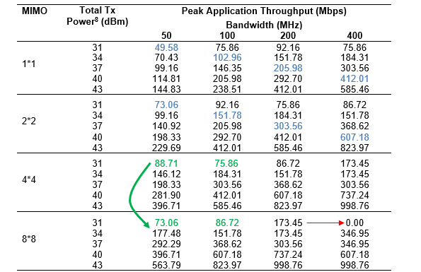
Table-13: Saturation throughput obtained for n261 band (gNB-UE distance of 100m, Rural macro pathloss) for various Bandwidth-MIMO-TxPower combinations. The blue entries show the doubling of throughput when power and BW is doubled. Red shows examples where throughput decreases with increase in bandwidth for fixed power and MIMO layers. Green entries are where throughput decreases with increase in MIMO layers, for fixed BW and power.
Discussion
In Table-13 we observe entries marked in:
Blue: When both the bandwidth and the power are doubled, with MIMO count kept constant, the peak throughput doubles. This is along expected lines.
Red: In the high bandwidth and low power regime, when the bandwidth is doubled with the transmit power and MIMO count held constant, the peak throughput does not increase but rather decreases.
Green: At low power when the MIMO layers are increased with fixed transmit power and bandwidth, the peak throughput surprisingly decreases.
Let us understand the red entries, i.e., throughput of 1*1 MIMO, 31 dBm Tx power for bandwidths of 200 and 400 MHz. We can simplify the PHY rate as equal to \(k \times L \times Q \times B \times R\) where\(\ k\) is some constant, \(L\ \)is the number of layers (set to 2 here), \(Q\) is the modulation order (2 in this case), \(R\ \)is the code rate and \(B\) is the bandwidth. From Table 10‑13 we see that when the bandwidth increases the spectral efficiency decreases due to an increase in thermal noise at higher bandwidths. The received power is constant since the transmit power is fixed. Since the drop in the MCS (due to the reduced spectral efficiency) is larger than the bandwidth increase - \(0.438 \times 200\ \)vs. \(0.188 \times 400\) - the net effect is a decline in the throughput.
BW (MHz) |
Rx Power (dB) |
Noise (KTB) |
SNR |
Spectral Efficiency |
Spec Eff Table cut off |
MCS Index |
MCS Code Rate |
R (Code rate/1024) |
Throughput (Mbps) |
|---|---|---|---|---|---|---|---|---|---|
200 |
-91.26 |
-90.81 |
-0.44 |
0.927 |
0.8770 |
3 |
449 |
0.438 |
92.21 |
400 |
-91.26 |
-87.80 |
-3.45 |
0.537 |
0.3770 |
1 |
193 |
0.188 |
75.92 |
Table-14: Rx Power, Noise, SNR, Spectral Efficiency obtained for different bandwidths with Tx power at 31 dBm.
Next, we turn to the green entries. In Table 10‑13 notice that when the MIMO layer count is increased from 4 to 8, the received power (per layer) decreases. This happens because the transmit power is equally divided among all the layers. As SNR reduces, the spectral efficiency per layer decreases. Since the MCS drop (due to lower spectral efficiency) is larger than the multiplexing gain got from multiple MIMO streams - \(4 \times 0.438\ \)vs \(8 \times 0.188\ \)- the consequence is a decrease in throughput.
MIMO Layers |
BW (MHz) |
Rx Power (dB) |
Noise (KTB) |
SNR |
Spec Efficiency |
Spec Eff Table cut off |
MCS Index |
MCS Code Rate |
R (Code rate/ 1024) |
Throughput (Mbps) |
|---|---|---|---|---|---|---|---|---|---|---|
4 |
50 |
-97.28 |
-96.83 |
-0.44 |
0.927 |
0.8770 |
3 |
449 |
0.438 |
88.76 |
8 |
50 |
-100.29 |
-96.83 |
-3.45 |
0.537 |
0.3770 |
1 |
193 |
0.188 |
73.11 |
Table-15: Rx Power, Noise, SNR, Spectral Efficiency obtained for each MIMO layer with Tx power set to 31 dBm.
Exercises
Estimate the data throughput analytically for different values of Transmit power, Bandwidth and MIMO layer count (Each student can be given a personalized experiment)
Understanding 5G NR (3GPP) pathloss models
Objective
In the elementary case of 1gNB communicating with 1UE over a 5G NR network, in a rural setting, we study the question: How does the UE-gNB pathloss vary with the distance between the UE and the gNB and the gNB height? What is the optimal height of a gNB?
Motivation
We start with a non-technical explanation of the objective. A mobile phone (in the hands of an individual) is the UE; the cell tower is the guns. Assume the person is in a rural area and is outdoors. Pathloss would determine the signal strength displayed on the phone; a higher loss means a lower signal strength. Mobile network operators (think of the top service providers in our country) invest large sums in setting-up the towers. They wish to know the tower height that gives users the highest signal strength. The answer is not obvious: the more the height of the gNB, the more likely it is that there exists a line-of-sight path to a given UE, but the signal has to traverse a longer distance, incurring a higher path loss. The cell radius might also play a role here: perhaps a lower height is better for smaller sized cells, and a greater height is better for large cells. In this experiment, we will understand these trade-offs.
The 5G pathloss equations
To answer these questions, we look at the 5G pathloss equations for a rural scenario as defined in the 3GPP 38.901 standards:
Scenario |
LOS/ NLOS State |
Pathloss (dB) (\(f_{c}\) in GHz and \(d\) in meters) |
Shadow Fading (σ) |
Parameter values and ranges |
|---|---|---|---|---|
Rural Macro |
LOS |
\[\begin{split}P{L_{RMA}}_{LOS} = \left\{ \begin{array}{r}
PL_{1},\ 10m \leq d_{2D} \leq d_{BP} \\
PL_{2},\ d_{BP} \leq d_{2D} \leq 10Km
\end{array} \right.\end{split}\]
\[PL_{2} = PL_{1}(d_{BP}) + 40\log_{10}{\left(\frac{d_{3D}}{d_{BP}}\right)}\]
|
\[\sigma_{SF} = 4\]
\[\sigma_{SF} = 6\]
|
\[h_{BS} = 35m\]
\[h_{UT} = 1.5m\]
\[W = 20m\]
\[h = 5m\]
\[5m \leq h \leq 50m\]
\[5m \leq W \leq 50m\]
\[10m \leq h_{BS} \leq 150m\]
\[1m \leq h_{UT} \leq 10m\]
|
NLOS |
\[P{L_{RMa}}_{NLOS} = max(P{L_{RMa}}_{LOS}, P{L_{RMa}}_{NLOS})\]
For \(10m \leq d_{2D} \leq 5Km\)
|
\[\sigma_{SF} = 8\]
|
||
NOTE: 1. Break point distance \(d_{BP} = 2\pi h_{BS}h_{UT}f_{c}/c\), where \(f_{c}\) is the centre frequency in Hz. \(c = 3.0*10^{8}\ \mathrm{m/s}\) is the propagation velocity in free space, and \(h_{BS}\) and \(h_{UT}\) are the antenna heights at the BS and the UT, respectively.
|
||||
Table-16: Pathloss equations for Rural Macro environment for LOS and NLOS states.

Figure-49: Definition of d2D and d3D

Figure-50: Definition of d2D-out, d2D-in and d3D-out, d3D-in for indoor UEs
Note that,
Observing the above equations, we see that the pathloss is not a simple expression in terms of gNB height. The other parameters affecting the pathloss are a) the UE-gNB 2D distance and b) the UE state .
Consequently, we investigate the revised question: how does the UE-gNB pathloss vary for combinations of gNB height, UE-gNB 2D distance, and UE states (LOS/NLOS)?
Network simulation setup
Open NetSim and click on Experiments > 5G NR > Understanding 5G NR (3GPP) pathloss models then click on the tile in the middle panel to load the example as shown in below.

Figure-51: List of Experiments
Network scenario:
NetSim UI would display the following network topology when you open the example configuration file as shown below screenshot.

Figure-52: Network topology in this experiment
Settings
The following settings were configured in the network setup.
The UE is placed 50m away from the gNB.
The following properties were set in Interface 5G RAN, Physical Layer of gNB.
gNB Interface 5G RAN |
|
|---|---|
gNB Height (m) |
Varied from 10 to 150 |
Tx Power (dBm) |
40 |
Tx Antenna Count |
2 |
Rx Antenna Count |
2 |
CA Type |
Single Band |
CA Configuration |
n78 |
DL: UL Ratio |
4:1 |
Numerology |
0 |
Channel Bandwidth (MHz) |
10 |
MCS Table |
QAM64 |
CQI Table |
TABLE1 |
Outdoor Scenario |
Rural Macro |
Indoor Office Type |
Mixed Office |
Pathloss Model |
3GPPTR38.901-7.4.1 |
LOS Mode |
User Defined |
LOS Probability |
0 or 1 (Varied) |
Shadow Fading Model |
None |
Fast Fading Model |
No Fading |
Table-17: gNB Interface RAN properties
Tx Antenna Count = Rx Antenna Count = 2 in UE > Interface 5G RAN > Physical Layer
A downlink CBR application was configured from Wired Node to UE with Packet Size 1460B and IAT 1168µs and the start time was set to 1s.
Run simulation for 2s.
In case 2, set the LOS probability to 0 and run simulation for various gNB heights.
In case 3, place the UE 1000m away from the gNB and repeat the above procedure.
In case 4, set the LOS probability to 0 and run simulation for 2s.
Click on the Log/Plots tab in the right panel toolbar to enable LTENR Radio measurement as shown in Figure-53.

Figure-53: Enabling the LTENR Radio measurement log
After the simulation, note down the Pathloss from the log file generated for various gNB heights.
Case 02: 5G NR 3GPP Pathloss Models Distance 500m
Grid setting is 1000m x1000m.
Distance between gNB and UE is 500m.
Case 03: 5G NR 3GPP Pathloss Models Distance 1000m
Grid setting is 2000m x2000m.
Distance between gNB and UE is 1000m.
Results
After simulation, open LTENR Radio measurement Log file from Netsim Result dashboard.

Figure-54: NetSim Results window
Note down the Pathloss value by filtering the channel to PDSCH, for each gNB height setting

Figure-55: NetSim LTENR Radio measurement Log file
Upon running simulations, we can obtain the following table below which contains pathloss values for:
gNB height varying from 10m to 150m in steps of 20m.
UE placed at 50m, 500m and 1000m away from gNB, and
UE states: LOS, NLOS
gNB Height(m) |
Pathloss (dB) |
|||||
|---|---|---|---|---|---|---|
UE 50m, LOS |
UE 50m, NLOS |
UE 500m, LOS |
UE 500m, NLOS |
UE 1 km, LOS |
UE 1km, NLOS |
|
10 |
77.73 |
92.39 |
98.71 |
132.47 |
105.58 |
144.61 |
30 |
78.87 |
84.04 |
98.73 |
120.54 |
105.58 |
132.21 |
50 |
80.58 |
82.57 |
98.76 |
115.30 |
105.59 |
126.73 |
70 |
82.35 |
82.72 |
98.80 |
111.92 |
105.60 |
123.16 |
90 |
83.99 |
83.99 |
98.86 |
109.45 |
105.62 |
120.51 |
110 |
85.45 |
85.45 |
98.93 |
107.52 |
105.64 |
118.41 |
130 |
86.75 |
86.75 |
99.02 |
105.96 |
105.66 |
116.68 |
150 |
87.91 |
87.91 |
99.12 |
104.66 |
105.69 |
115.20 |
Table-18: Pathloss values for various combinations. The gNB heights are shown in Column 1. Other columns show the gNB-UE 2D distance (50m, 500m and 1Km) and the UE state (LOS/NLOS)
Numerical verification of two cases
In this section we numerically calculate the pathloss per the 5G pathloss formula for two cases to verify NetSim’s output.
Symbol |
Description |
Value |
|
|---|---|---|---|
\[\mathbf{d}_{\mathbf{BP}}\]
|
\[Breakpoint\ distance\]
|
||
\[\mathbf{h}_{\mathbf{BS}}\]
|
\[Height\ of\ Base\ Station\]
|
\[10m\]
|
|
\[\mathbf{h}_{\mathbf{UT}}\]
|
\[Height\ of\ UE\]
|
\[1.5m\]
|
|
\[\mathbf{f}_{\mathbf{c}}\]
|
\[Central\ Frequency\ in\ Hz\]
|
\[3550*10^{6}Hz = 3.55GHz\]
|
|
\[\mathbf{c}\]
|
\[Speed\ of\ light\]
|
\[3*10^{8}m/s\]
|
|
\[\mathbf{W}\]
|
\[Street\ width\]
|
\[20m\]
|
|
\[\mathbf{h}\]
|
\[Building\ Height\]
|
\[5m\]
|
|
Table-19: Various parameters used in the pathloss calculations and their values
Case 1: gNB height = 10m, UE State is LOS and UE-gNB 2D Distance = 50m
Breakpoint Distance:
Pathloss Calculation
If \((10 \leq d_{2D} \leq d_{BP})\)
- \(PL1\ = \ (20\ *\ log10(40\ *\ PI\ *\ distance3D\ *\ fc_{(GHz)}\ /\ 3))\ + \ fmin((0.03\ *\ pow(h,\ 1.72)),\ 10)\ *\ \ log10(distance3D)\)
\(\quad - \ fmin((0.044\ *\ pow(h,\ 1.72)),\ 14.77)\ + \ (0.002\ *\ log10(h)\ *\ distance3D)\)
- \(\mathbf{=}\left( 20*log_{10}\left( 40*3.14*50.71*\frac{3.55}{3} \right) \right) + f_{\min}\left( \left( 0.03*pow(5,1.72) \right),10 \right)*log_{10}(50.71)\)
\(\quad - f_{\min}\left( \left( 0.044*pow(5,1.72) \right),14.77 \right) + \left( 0.002*log_{10}(5)*50.71 \right)\mathbf{=}77.73\ dB\)
Pathloss = 77.73 dB (matches NetSim result)
Case 2: gNB height = 10m, UE State is NLOS and UE-gNB 2D Distance = 50m
Breakpoint Distance:
Pathloss Calculation
If \((10 \leq d_{2D} \leq 5Km)\)
Where,
- \(PL_{NLOS} = 161.04 - 7.1{*\log}_{10}(W) + 7.5*\log_{10}{(h)} - \left( 24.37 - 3.7*\left( \frac{h}{h_{BS}} \right)^{2} \right)*\log_{10}{\left( h_{BS} \right)}\)
\(\quad + (43.42 - (3.1*\log_{10}{(h_{BS})})*(\log_{10}{\left( d_{3D} \right)}) - 3) + 20*(\log_{10}{(f_{c})}) - (3.2*(\log_{10}{\left( 11.75*h_{UT} \right)})^{2}) - 4.97\)
- \(= 161.04 - (7.1*\log_{10}{(20)}) + 7.5*(\log_{10}(5)) - (24.37 - 3.7*\left( \frac{5}{10} \right)^{2})*(\log_{10}{(10)}) + (43.42 - (3.1*\log_{10}{(10)})*(\log_{10}{(50.71)}) - 3)\)
\(\quad + 20*(\log_{10}{(3.55)}) - (3.2*(\log_{10}{\left( 11.75*1.5 \right)})^{2}) - 4.97 = 92.39\ dB\)
- \(PL_{LOS}\ = \ (20\ *\ log10(40\ *\ PI\ *\ distance3D\ *\ fc_{(GHz)}\ /\ 3))\ + \ fmin((0.03\ *\ pow(h,\ 1.72)),\ 10)\ *\ \ log10(distance3D)\)
\(\quad - \ fmin((0.044\ *\ pow(h,\ 1.72)),\ 14.77)\ + \ (0.002\ *\ log10(h)\ *\ distance3D)\)
- \(\mathbf{=}\left( 20*log_{10}\left( 40*3.14*50.71*\frac{3.55}{3} \right) \right) + f_{\min}\left( \left( 0.03*pow(5,1.72) \right),10 \right)*log_{10}(50.71)\)
\(\quad - f_{\min}\left( \left( 0.044*pow(5,1.72) \right),14.77 \right) + \left( 0.002*log_{10}(5)*50.71 \right)\mathbf{=}77.73\ dB\)
Pathloss = 92.39 dB (matches NetSim result)

Figure-56: Plots of Pathloss vs. gNB height for different UE-gNB 2D Distances and UE States (LOS, NLOS)
Discussion
We explain the results in the plots above from the specifics of the pathloss formulas.
In the LOS plots, the pathloss is flat for different gNB heights when the gNB-UE distance is high, i.e 500m and 1 km. When the gNB-UE distance is low i.e 50m, the pathloss increases with gNB height.
Observe from the LOS pathloss formula that pathloss is proportional to \(\log{(D_{3d})}\). \(D_{3d}\) of the 3D distance between the UE and the gNB and is defined as \(d_{3D} = \sqrt{\left( d_{2D} \right)^{2} + \left( h_{BS} - h_{UT} \right)^{2}}\). It is the hypotenuse of the right triangle with the base being the gNB-UE 2D distance.
Since the length of the hypotenuse is sensitive to the height of the triangle, when the base is small, we see the pathloss increasing with gNB height when the UE is 50m away.
Inversely, the length of the hypotenuse is almost insensitive to the triangle height when the base is much larger than the height. Therefore, when the UE is far, the gNB’s height does not have a noticeable impact. Pathloss is flat when the UE is 500m and 1 km away.
Let us turn to the NLOS results.
The NLOS pathloss decreases with gNB height when the gNB-UE distance is high i.e 500m and 1000m.
When the UE is near, i.e 50m, the NLOS pathloss first decreases and then increases with gNB height.
The reason for this kind of variation is the NLOS pathloss formulas in which that pathloss has terms proportional to:
\(\log\left( h_{BS} \right)\), \({\log{(\left( h_{BS} \right)}}^{2})\)
\(\log{(d_{3d})}\)
The reciprocal of \(\left( h_{BS} \right)^{2}\ \)
We see that at larger distances LOS pathloss is almost flat and NLOS pathloss decreases, as gNB height increases. From the plots one sees that the optimal gNB height would be between 125m to 150m in the example discussed above.
Exercises
Make a separate plot with the UE distance on the X-axis and show the behavior for three different values of the gNB height. Recommend the gNB height for different cell radii. Does your recommendation make practical sense?
Use MATLAB or Python to plot similar curves from the standard pathloss formulas. Compare your results against the NetSim results.
(For the Instructor or TA) Generate personalized exercises where the student can be asked to
Recommend the gNB height given the cell radius
Recommend gNB height given the transmit power.
Find the cell radius given the gNB height, transmit power and noise figure
Performance of OFDMA SU-MIMO in 5G
The 5G cellular system utilizes OFDMA MIMO technology at the physical layer. This technology permits degrees of freedom in frequency, time, and “space” for multiplexing the data of multiple users. Let us consider the downlink direction, i.e., from the base-station (gNB) to the users (UE). The system bandwidth (e.g., 100 MHz), has several OFDM carriers, separated by a carrier spacing (e.g., 60 KHz, yielding 132 physical resource blocks (PRBs) or carriers ). Each PRB has 12 consecutive sub carriers. These carriers (set of usable PRBs) have time-division framing (e.g., 0.25 ms), each frame carrying 14 symbols of which 18% on average is modeled as overheads in NetSim. When the above system is used to carry data to multiple users, it is called OFDMA. In addition, MIMO technology exploits spatial multiplexing, thereby effectively carrying multiple (spatially multiplexed) symbols for each time-symbol in the OFDM carrier. In MIMO all the spatially multiplexed symbols for an OFDM symbol can be destined to one user, in which case it is called Single User MIMO, or SU-MIMO.
In this experiment we study the performance of OFDMA along with SU-MIMO to carry downlink data to multiple UEs. Since we have SU-MIMO, multiple users are multiplexed by OFDMA, and SU-MIMO is used to obtain spatial multiplexing gain, depending on the number of antennas available at the UE. In Multi User MIMO (MU-MIMO) different spatial layers within the same resource block, can be allotted to different UEs.
Objective
Simulate a maximum data transmission rate , using OFDMA and SU-MIMO, for the following 4 cases
1 gNB with 8 Tx antennas transmitting to 1 UE with 8 Rx antennas using all the 132 resource blocks
1 gNB with 8 Tx antennas transmitting to 2 UEs each with 4 Rx antennas, each using \(\frac{132}{2}\) resource blocks on average
1 gNB with 8 Tx antennas transmitting to 4 UEs each with 2 Rx antennas, each using \(\frac{132}{4}\) resource blocks on average,
1 gNB with 8 Tx antennas transmitting to 8 UEs each with 1 Rx antennas, each using \(\frac{132}{8}\) resource blocks on average
Repeat the above cases with the number of UEs now set to 1 for each case, while the antenna counts remain the same. Show that there is no difference in maximum capacity between a single user and a multi-user transmission, when using SU-MIMO. And finally, explain the results obtained for different number of receive antennas by using matrix theory to compute the eigen values of the associated Gram matrices.
Introduction
We begin with a description of the channel model. Consider a transmitter with \(N_{t}\) transmit antennas, and a receiver with \(N_{r}\)receive antennas. The channel can be represented by the \(N_{r} \times N_{t}\) matrix \(\mathbf{H}\) of channel gains \(h_{ij}\) representing the gain from transmit antenna \(j\ \)to receive antenna \(i.\) The \(N_{r}\ \times \ 1\) received signal \(\mathbf{y}\) is equal to
The channel state information is the channel matrix \(\mathbf{H}\) and/or its distribution.
Under rich scattering conditions the MIMO channel can be decomposed into parallel non-interfering channels. The number of such parallel streams is known as the layer count and is equal to \(\ Min(N_{t},\ N_{r})\). These parallel channels are commonly referred to as the eigenmodes of the channel because the singular values of \(\mathbf{H}\) are equal to the square root of the eigenvalues of the Wishart matrix \(W = H\ H^{\dagger}\) (for \(N_{t} \geq N_{r}\)).
Since each layer is reduced to a flat fading SISO channel, i.e., for layer \(j,\ 1 \leq j \leq LayerCount\),
where, \(x_{j}\) is the symbol transmitted, \(\lambda_{j}\) is the corresponding eigenvalue of the Wishart matrix obtained as in the previous section, \(w_{j}\) is circular symmetric complex Gaussian noise, and \(y_{j}\) is the complex valued baseband received symbol.
If fast fading with eigen-beamforming is enabled in NetSim’s GUI, then the MIMO link is modelled by parallel SISO channels with the symbol level beamforming gain derived from the eigenvalues of the Wishart matrix.
Three assumptions made in NetSim are:
A1. Perfect CSIT and CSIR: The channel matrix \(\mathbf{H}\) is assumed to be known perfectly, at the start of each frame, at the transmitter and receiver, respectively. With perfect CSIT the transmitter can adapt its transmission rate (MCS) relative to the instantaneous channel state (SNR).
A2. No channel errors.
A3. The transmit power is equally split between all layers transmitted. The justification lies in the fact that at a high SNR, (iterative) water-filling will lead to nearly equal power allocation across all subcarriers and all layers.
Note that the LOS probability parameter in NetSim is solely used to compute the large scale pathloss per the 3GPP 38.901 standard. This parameter is not used in the channel rank (MIMO layers) computations. The Fading and Beam Forming parameter is used to determine (i) the number of MIMO layers and (ii) the gains in each layer, as shown in the table below.
Parameter drop down option |
No. of MIMO layers |
Beamforming Gain |
|---|---|---|
No fading MIMO unit gain |
Min \({(N}_{t},\ N_{r})\) |
Unity (0 dB) |
No fading MIMO array gain |
Min \({(N}_{t},\ N_{r})\) |
Max \({(N}_{t},\ N_{r})\) |
Rayleigh with Eigen Beamforming |
Min \({(N}_{t},\ N_{r})\) |
Eigen values of the Wishart Matrix |
Table-20: Gains at different layers
Network simulation setup
Open NetSim and click on Experiments > 5G NR > Performance of OFDMA SU-MIMO in 5G then click on the tile in the middle panel to load the example as shown in below.

Figure-57: List of Experiments
NetSim Settings
The following parameters were configured in Interface 5G RAN- Physical Layer of gNB and UE:
gNB- Interface 5G_RAN Parameters |
|
|---|---|
gNB Height |
10m |
Tx Power |
40 dBm |
Duplex Mode |
TDD |
CA Type |
SINGLE BAND |
CA Configuration |
n78 |
DL: UL Ratio |
4:1 |
Numerology |
2 |
Channel Bandwidth (MHz) |
100 |
Tx Antenna Count |
8 |
Rx Antenna Count |
1 |
MCS Table |
QAM256 |
CQI Table |
TABLE2 |
Pathloss Model |
3GPPTR38.901-7.4.1 |
Outdoor Scenario |
Urban Macro |
LOS NLOS Selection |
User Defined |
LOS Probability |
1 |
Shadow Fading Model |
None |
Fast Fading Model |
Rayliegh |
Channel Rank/ MIMO layers |
Max Rank |
MIMO Beamforming Model |
Eigen BF |
Coherence Time (ms) |
10 |
Additional Loss Model |
None |
UE Interface 5G RAN |
|
Tx Power |
23 dBm |
UE Height |
1.5m |
Tx Antenna Count |
1 |
Rx Antenna Count |
<varied> |
Table-21: gNB and UE properties
The following parameters were configured in the wired link properties:
Wired Link Parameters |
|
|---|---|
Wired Link Speed |
10 Gbps |
Wired Link BER |
0 |
Wired Link Propagation Delay |
5 µs |
Table-22: Wired link properties
Run simulation for 1.1s.
Case 1: 1 gNB - 8 Tx antennas, 1 UE - 8 Rx antennas
Network Scenario:

Figure-58: Network topology in this experiment
Additional Settings:
The Tx Antenna Count was set to 1 and Rx Antenna Count was set to 8 in Interface 5G RAN- Physical Layer in the UE
The following parameters were set in Application Properties:
Application Parameters |
|
|---|---|
Application |
CBR |
Packet Size |
1460 |
Inter Packet Arrival Time (µs) |
3.33 |
Start Time |
1 |
Transport Protocol |
UDP |
Table-23: Application properties
Result:
Application |
Throughput (Mbps) |
|---|---|
App_1_CBR |
1959.55 |
Table-24: Throughput obtained per UE
Case 2: 1 gNB- 8 Tx antennas, 2 UEs with 4 Rx antennas each
Network Scenario:

Figure-59: Network topology in this experiment
Additional Settings:
The Tx Antenna Count was set to 1 and Rx Antenna Count was set to 4 in Interface 5G RAN- Physical Layer in both the UEs.
The following parameters were set in Application Properties:
Application Parameters |
||
|---|---|---|
Wired Node- UE_10 |
Wired Node- UE_11 |
|
Application |
CBR |
CBR |
Packet Size |
1460 |
1460 |
Inter Packet Arrival Time (µs) |
12.97 |
12.97 |
Start Time |
1 |
1 |
Transport Protocol |
UDP |
UDP |
Table-25: Application properties
Result:
Throughput Obtained (Mbps) |
||
|---|---|---|
UE_10 |
UE_11 |
Aggregate Throughput (Mbps) |
685.26 |
659.92 |
1345.18 |
Table-26: Throughput obtained per uE
Case 3: 1 gNB 8- Tx antennas, 4 UEs with 2 Rx antennas each
Network scenario:

Figure-60: Network topology in this experiment
Additional Settings:
The Tx Antenna Count was set to 1 and Rx Antenna Count was set to 2 in Interface 5G RAN- Physical Layer in all the UEs.
The following parameters were set in Application Properties:
Application Parameters |
||||
|---|---|---|---|---|
Wired Node- UE_8 |
Wired Node- UE_9 |
Wired Node- UE_10 |
Wired Node- UE_11 |
|
Application |
CBR |
CBR |
CBR |
CBR |
Packet Size |
1460 |
1460 |
1460 |
1460 |
Inter Packet Arrival Time (µs) |
53.09 |
53.09 |
53.09 |
53.09 |
Start Time |
1 |
1 |
1 |
1 |
Transport Protocol |
UDP |
UDP |
UDP |
UDP |
Table-27: Application properties
Result:
Throughput (Mbps) |
||||
|---|---|---|---|---|
UE_10 |
UE_11 |
UE_12 |
UE_13 |
Aggregate Throughput (Mbps) |
199.14 |
199.84 |
198.09 |
200.54 |
797.61 |
Table-28: Throughputs obtained per UE
Case 4: 1 gNB 8 tx antennas, 8 UEs with 1 Rx antennas each
Network Scenario:

Figure-61: Network topology in this experiment
Additional Settings:
The Tx Antenna Count was set to 1 and Rx Antenna Count was set to 1 in Interface 5G RAN- Physical Layer in all the UEs.
The following parameters were set in Application Properties:
Application Parameters |
||||||||
|---|---|---|---|---|---|---|---|---|
Wired Node- UE_10 |
Wired Node- UE_11 |
Wired Node- UE_12 |
Wired Node- UE_13 |
Wired Node- UE_14 |
Wired Node- UE_15 |
Wired Node- UE_16 |
Wired Node- UE_17 |
|
Application |
CBR |
CBR |
CBR |
CBR |
CBR |
CBR |
CBR |
CBR |
Packet Size |
1460 |
1460 |
1460 |
1460 |
1460 |
1460 |
1460 |
1460 |
Inter Arrival Time (µs) |
212.36 |
212.36 |
212.36 |
212.36 |
212.36 |
212.36 |
212.36 |
212.36 |
Start Time |
1 |
1 |
1 |
1 |
1 |
1 |
1 |
1 |
Transport Protocol |
UDP |
UDP |
UDP |
UDP |
UDP |
UDP |
UDP |
UDP |
Table-29: Application properties
Results:
Throughput Obtained (Mbps) |
||||||||
|---|---|---|---|---|---|---|---|---|
UE_10 |
UE_11 |
UE_12 |
UE_13 |
UE_14 |
UE_15 |
UE_16 |
UE_17 |
Aggregate Throughput (Mbps) |
51.98 |
52.79 |
52.09 |
52.21 |
53.03 |
50.22 |
51.63 |
51.63 |
415.57 |
Table-30: Throughputs obtained per UE
Discussion
We combine the results of the four cases and present it in the table below.
Rx Antenna Count per UE |
Throughput (Mbps) |
Aggregate Throughput (Mbps) |
|||||||
|---|---|---|---|---|---|---|---|---|---|
UE_1 |
UE_2 |
UE_3 |
UE_4 |
UE_5 |
UE_6 |
UE_7 |
UE_8 |
||
8 |
1959.55 |
1959.55 |
|||||||
4 |
685.26 |
659.92 |
1345.18 |
||||||
2 |
199.14 |
199.84 |
198.09 |
200.54 |
797.61 |
||||
1 |
52.79 |
52.09 |
50.92 |
52.79 |
51.62 |
52.44 |
52.91 |
52.20 |
417.76 |
Table-31: Throughput comparison table for different Rx Antenna Counts
We compare the aggregate throughputs (from Table-31) with single UE peak throughputs.
UE Rx Antenna Count per UE |
Aggregate Throughput (Mbps) |
Single UE Peak Throughput (Mbps) |
|---|---|---|
8 |
1936.54 (1 UE 8 Rx Antennas) |
1936.54 (1 UE 8 Rx Antennas) |
4 |
1352.89 (2 UEs with 4 Rx Antennas) |
1330.46 (1 UE 4 Rx Antennas) |
2 |
786.65 (4 UEs with 2 Rx Antennas) |
754.52 (1 UE 2 Rx Antennas) |
1 |
418.49 (8 UEs with 1 Rx Antennas) |
414.75 (1 UE 1 Rx Antennas) |
Table-32: Throughputs obtained for different Rx Antenna counts in multi and single UE cases.
From Table-32 it becomes clear that the bandwidth is shared across the UEs by OFDMA. It is just like having one UE use the entire bandwidth.
Theoretical analysis:
8*8 SU-MIMO
\(2^{k}\) carriers in the OFDMA system
\(S:\ \)symbol rate per carrier (assuming the same numerology for all carriers)
\(L:\ \)is the large-scale pathloss, including shadowing (not including the fading). Note that, \(L\) is modelled as \(c\left( \frac{d}{d_{0}} \right)^{- \eta}\) where \(\eta\) is the pathloss coefficient.
Then the expected rate to the single SU-MIMO user is given by
where \(P_{j}\) is the power allotted to the \(j^{th}\) equivalent channel, with \(\sum_{j = 1}^{8}{P_{j} = P,\ }\) the total transmit power. We assume equal power allocation, so that \(P_{j} = \frac{P}{8},\ \) so that
8*1 SU-MIMO, with 8 such UEs
\(2^{k - 3}\) OFDMA carriers per UE
Then, for the same OFDMA symbol rate, \(S,\ \) and large-scale pathloss, \(L,\) the total expected rate for the 8 UEs is given by:
From matrix theory we know that the sum of the eigenvalues of a matrix is equal to its trace. Therefore
We know that when\(\ a,\ \lambda_{1},\ \lambda_{2} > 0\)
and by monotonicity of log function, it follows that
Extending this inequality recursively, we get
Using the above expressions, we can compare the expected total downlink throughputs for one 8x8 SU-MIMO UE, with eight 8x1 SU-MIMO UEs, as follows:
where the first inequality arises from the argument given earlier, and the second equality follows from the equality between the trace of a matrix and the sum of its eigenvalues. Physically, the first inequality captures the performance gain obtained by splitting the power over the different spatial degrees of freedom. The second inequality follows from the fact the fact that the logarithm function is concave and by an application of Jensen’s inequality. We see from Table-31 that \(\mathbb{E}R_{1} = 1942.26\ Mbps,\ \)whereas \(\mathbb{E}R_{2} = 418.46\ Mbps\), showing the large effect of the two inequalities in the above argument.
Exercises
Carefully explain your observations. Also, place the UEs at different distances from the gNB and see how the throughput changes. Again, explain your observations.
Vary the height of UEs (as this also effects pathloss) and see how the throughput changes. Again, explain your observations.
5G Numerologies and their impact on end-to-end latencies
Objective
5G NR supports flexible numerology with a range of subcarrier spacings, based on scaling a baseline subcarrier spacing of 15 kHz to support diverse spectrum bands/types and deployment models. The numerology, \(\mu\), can take values from 0 to 4 and specifies the Sub-Carrier Spacing (SCS) as \(15 \times 2^{µ}\) kHz and a slot length of \(\frac{1}{2^{µ}}\) ms. With \(\mu\) varying from 0 to 4, Sub-Carrier Spacing (SCS) varies from 15 to 240 kHz.
We investigate the impact of numerology on latency and throughput in two cases
A simple case where one UE is transmitting and receiving UDP traffic from a server
A complex 5G scenario with Sensors, Cameras and Smartphones having DL and UL, TCP and UDP flows.
Theory
In NetSim, for data channels FR1 supports \(\mu = 0,\ 1,\ 2\) and FR2 supports \(\mu = 2,\ 3\). The setting \(\mu = 0\) corresponds to the LTE (4G) system configuration. In the time domain (to support backwards compatibility with LTE) the frame length in 5G NR is set to 10 ms, and each frame is composed of 10 subframes of 1 ms each. The 1 ms subframe is then divided into one or more slots in 5G, whereas LTE had exactly two slots in a subframe. The slot size is defined based on \(\mu\), and the number of slots is \(2^{\mu}\). The number of OFDM symbols per slot is 14 for a configuration using normal cyclic prefix. For extended cyclic prefix, the number of OFDM symbols per slot is 12.

Figure-62: Frame, subframe and slot structure for different numerologies
For \(\mu = 0\) there are 1 slot per subframe, for \(\mu = 1\) there are 2 slots per subframe, for \(\mu = 2\) there are 4 slots per subframe and so on. The number of slots per frame is ten times of number of slots per sub frame. Hence for \(\mu = 2\), there are 40 slots/frame.
Numerology |
Sub-Carrier Spacing (KHz) |
OFDM Symbols per Slot |
Slots per Frame |
Slots per Sub-frame |
|---|---|---|---|---|
0 |
15 |
14 |
10 |
1 |
1 |
30 |
14 |
20 |
2 |
2 |
60 |
14 |
40 |
4 |
3 |
120 |
14 |
80 |
8 |
4 |
240 |
14 |
160 |
16 |
Table-33: Table 1 1:Sub-carrier spacing, number of OFDM symbols per slot, slots
Network simulation setup
Open NetSim and click on Experiments > 5G NR > 5G Numerologies and their impact on end-to-end latencies then click on the tile in the middle panel to load the example as shown in below.

Figure-63: List of Experiments
Network Model
Case 1: One UE is transmitting and receiving UDP traffic from a server
This is a simple scenario whereby the UE is transmitting and receiving UDP traffic from a server as shown in Figure-64.

Figure-64: Network scenario. a) The RAN with a User Equipment b) 5G Core and C) Cloud Server. The device in the RAN has both UL and DL communication with the cloud server.
The UE connects to the gNB which connects to the 5G core. The 5G core then connects to the remote server over the cloud (represented by the router and WAN links).
Keeping all other parameters fixed, we vary the numerology μ, as 0, 1, 2 and see its impact on end-to-end latency and application (user) throughput. In terms of application data traffic, the User Equipment (UE) has two UDP flows, one Uplink and one Downlink, that goes in the UL towards a remote node on the Internet. These flows are fixed-rate flows:
Procedure
For the above scenario set the following properties:
gNB Properties -> Interface (5G_RAN) |
|
|---|---|
Pathloss Model |
None |
Frequency Range |
FR1 |
CA Type |
Single Band CA |
CA Configuration |
n78 |
Numerology |
0,1 and 2 |
Channel Bandwidth |
10 MHz |
DL: UL Ratio |
1:1 |
MCS Table |
QAM64 |
CQI Table |
Table 1 |
Table-34:The Physical Layer properties set in 5G RAN interface of gNB
Link Properties (All wired links) |
|
|---|---|
Uplink/ Downlink Speed (Mbps) |
10000 |
Uplink/ Downlink BER |
0 |
Uplink/ Downlink Propagation Delay (µs) |
0 |
Table-35:Wired Link properties set in this experiment
CUSTOM UL UDP |
|
|---|---|
Generation Rate (Mbps) |
5.8 |
Transport Protocol |
UDP |
Application Type |
Custom |
Start time (s) |
1 |
Packet Size (Bytes) |
1460 |
IAT Distribution |
Exponential |
Inter Arrival Time (μs) |
2000 |
Table-36: Custom application properties for UL UDP
CUSTOM DL UDP |
|
|---|---|
Generation Rate (Mbps) |
5.8 |
Transport Protocol |
UDP |
Application Type |
Custom |
Start time (s) |
1 |
Packet Size (Bytes) |
1460 |
IAT Distribution |
Exponential |
Inter Arrival Time (μs) |
2000 |
Table-37:Custom application properties for DL UDP
The Tx Antenna Count was set to 2 and Rx Antenna Count was set to 2 in gNB > Interface 5G_RAN >Physical Layer.
The Tx Antenna Count was set to 2 and Rx Antenna Count was set to 2 in UE > Interface 5G_RAN >Physical Layer.
Run simulation for 10 sec. After simulation completes go to metrics window and note down throughput and delay value from application metrics.
Case 2: A complex 5G scenario with Sensors, Cameras and Smartphones having DL and UL, TCP and UDP flows
To model a real-world scenario, we base our simulation on the setup shown in Figure-75. The link between the gNB and the L2_Switches that represents the Core Network (CN) is made with a point-to-point 10 Gb/s link, without propagation delay. The Radio Area Network (RAN) is served by 1 gNB, in which different UEs share the connectivity. We have 25 smartphones, 6 sensors, and 3 IP cameras. The bandwidth is 100MHz and Round Robin MAC Scheduler.

Figure-65: Network scenario. a) Cloud servers b) 5G Core and C) The RAN with 25 smartphones, 6 sensors and 3 cameras communicating. The devices in the RAN communicate with respective cloud servers for both Downloads and Uploads.
In terms of data traffic, the camera (video) and sensor nodes have one UDP flow each, that goes in the UL towards a remote node on the Internet. These flows are fixed-rate flows: we have a continuous transmission of 5 Mb/s for the video nodes, to simulate a 720p24 HD video, and the sensors transmit a payload of 500 bytes each 2.5 ms, that gives a rate of 1.6 Mb/s. For smartphones, we use TCP as the transmission protocol. These connect to database servers. Each phone downloads a 25MB file and uploads a 1.5MB file. These flows start at different times: the upload starts at a random time between the 4.5th and the 105th simulation seconds, while each download starts at a random time between the 1.5th and the 105th simulation seconds.
Flows (No of devices) |
Traffic Rate (Mbps) |
Segment / File Size (B) |
Traffic Dir. |
TCP ACK Dir. |
|
|---|---|---|---|---|---|
Camera (UDP) |
3 |
5 |
500 |
UL |
-- |
Sensor (UDP) |
6 |
1.6 |
500 |
UL |
-- |
Smartphone Upload (TCP) |
25 |
-- |
1,500,000 |
UL |
DL |
Smartphone Download (TCP) |
25 |
-- |
25,000,000 |
DL |
UL |
Table-38:Various parameters of the Traffic flow model for all the devices.
The numerology \(\ \mu\) can take values from 0 to 3 and specifies an SCS of \(15 \times 2^{\mu}\) kHz and a slot length of \(\frac{1}{2^{\mu}}\) ms. FR1 support \(\mu = 0,\ 1\) and \(2\), while FR2 supports \(\mu = 2,\ 3.\ \)We study the impact of different numerologies, and how they affect the end-to-end performance. The metrics measured and analyzed are a) Throughput of TCP uploads and b) Latency of the UDP uploads and downloads.
Procedure
For the above scenario set the following properties:
gNB Properties -> Interface (5G_RAN) |
|
|---|---|
Pathloss Model |
None |
Frequency Range |
FR1 |
CA Type |
Inter Band CA |
CA Configuration |
CA_2DL_2UL_n40_n41 |
CA1 |
|
Numerology |
0, 1 and 2 |
Channel Bandwidth |
50 MHz |
DL: UL Ratio |
1:4 |
CA2 |
|
Numerology |
0, 1 and 2 |
Channel Bandwidth |
50 MHz |
DL: UL Ratio |
1:4 |
MCS Table |
QAM64 |
CQI Table |
Table 1 |
Table-39: The Physical Layer properties set in 5G Ran interface of gNB
Phone UL TCP |
|
|---|---|
Application Type |
FTP |
Transport Protocol |
TCP |
Start Time (s) |
\[4.5 + 4(i - 1)where,\ i = 1,2,\ldots.25\]
|
Stop Time (s) |
105 |
File Size (B) |
1,500,000 |
Inter Arrival Time (μs) |
200 (simulation ends at 100s and hence only one file is sent) |
Table-40: Phone applications for UL TCP
Link Properties (All wired links) |
|
|---|---|
Uplink/ Downlink Speed (Mbps) |
10000 |
Uplink/ Downlink BER |
0 |
Uplink/ Downlink Propagation Delay (μs) |
5 |
Table-41: Wired link properties set in this experiment
Sensor UL UDP |
|
|---|---|
Generation Rate (Mbps) |
1.6 |
Transport Protocol |
UDP |
Application Type |
Custom |
Packet Size (Bytes) |
500 |
Inter Arrival Time (μs) |
2500 |
Table-42: Sensor application properties for UL UDP
Camera UL UDP |
|
|---|---|
Generation Rate (Mbps) |
5 |
Transport Protocol |
UDP |
Application Type |
Custom |
Packet Size (Bytes) |
500 |
Inter Arrival Time (μs) |
800 |
Table-43:Camera application properties for UL UDP
Phone DL TCP |
|
|---|---|
Application Type |
FTP |
Transport Protocol |
TCP |
Start Time (s) |
\[1.5 + 4(i - 1)where,\ i = 1,2,\ldots.25\]
|
Stop Time (s) |
105 |
File Size (B) |
25,000,000 |
Inter Arrival Time (μs) |
200(simulation ends at 100s and hence only one file is sent) |
Table-44: Phone application properties for DL TCP
The Tx Antenna Count was set to 2 and Rx Antenna Count was set to 2 in gNB > Interface 5G_RAN >Physical Layer.
The Tx Antenna Count was set to 2 and Rx Antenna Count was set to 2 in UE > Interface 5G_RAN >Physical Layer.
Run simulation for 110 sec. After simulation completes go to metrics window and note down throughput and delay value from application metrics.
Results
Case 1:
Application Type |
Throughput (Mbps) |
||
|---|---|---|---|
Numerology, \(\mathbf{\mu = 0}\) |
Numerology, \(\mathbf{\mu = 1}\) |
Numerology, \(\mathbf{\mu = 2}\) |
|
Custom DL (UDP) |
5.76 |
5.77 |
5.77 |
Custom UL (UDP) |
5.82 |
5.82 |
5.82 |
Table-45: Throughputs obtained for UL and DL UDP flows when numerology is varied from 0 to 2.
Application Type |
Delay (ms) |
||
|---|---|---|---|
Numerology, \(\mathbf{\mu} = \mathbf{0}\) |
Numerology, \(\mathbf{\mu} = \mathbf{1}\) |
Numerology, \(\mathbf{\mu} = \mathbf{2}\) |
|
Custom DL (UDP) |
2.000 |
1.032 |
0.583 |
Custom UL (UDP) |
1.997 |
1.003 |
0.577 |
Table-46: Delay obtained for UL and DL UDP applications when numerology is varied from 0 to 2.

Figure-66: Custom DL and UL throughput vs numerology. Numerology has no impact on throughput

Figure-67: Custom DL and UL delay vs numerology. The delay for both DL and UL decreases as numerology is increased
Case 2:
Application Type |
Average Throughput (Mbps) |
||
|---|---|---|---|
Numerology, \(\mathbf{\mu = 0}\) |
Numerology, \(\mathbf{\mu = 1}\) |
Numerology, \(\mathbf{\mu = 2}\) |
|
Camera Video UL (UDP) |
4.99 |
4.99 |
4.99 |
Sensor UL (UDP) |
1.59 |
1.59 |
1.59 |
Smartphone UL (TCP) |
86.29 |
172.52 |
311.40 |
Smartphone DL (TCP) |
101.67 |
156.43 |
151.74 |
Table-47: Average and aggregate throughputs obtained for Camera, Sensors and Smartphones, when numerology is varied from 0 to 2.
Application Type |
Average Delay (ms) |
||
|---|---|---|---|
Numerology, \(\mathbf{\mu} = \mathbf{0}\) |
Numerology, \(\mathbf{\mu} = \mathbf{1}\) |
Numerology, \(\mathbf{\mu} = \mathbf{2}\) |
|
Camera Video UL (UDP) |
1.82 |
0.92 |
0.47 |
Sensor UL (UDP) |
2.28 |
1.52 |
0.77 |
Smartphone UL (TCP) |
79.73 |
39.98 |
21.84 |
Smartphone DL (TCP) |
992.32 |
643.28 |
660.70 |
Table-48: Average delay obtained for Camera, Sensors and Smartphones, when numerology is varied from 0 to 2

Figure-68: The average uplink throughputs for Cameras and Sensors remains the same as the numerology is increased. This is because the flow is UDP.

Figure-69: The average uplink delays for cameras and sensors decreases as the numerology is increases

Figure-70: The average throughput for smartphone downlink and uplink increases with numerology. This is because the flow is TCP

Figure-71: The average delay for smartphone downlink and uplink decreases with numerology. This is because the flow is TCP.
Discussion
For UDP applications, the Numerology, μ does not impact the throughput.
The TCP throughput is inversely proportional to round trip time. Therefore, for applications running over TCP the throughput increases with higher numerology since a higher Numerology leads to reduced round-trip times.
Therefore, the selection of the numerology in an NR system should be carefully made by considering the traffic patterns.
References
Patriciello, N., Lagen, S., Giupponi, L., & Bojovic, B. (2018). 5G New Radio Numerologies and their Impact on the End-To-End Latency. IEEE 23rd International Workshop on Computer Aided Modeling and Design of Communication Links and Networks (CAMAD).
MIMO Communication: Channel Matrix Asymptotic Analysis
Objective
In this experiment, properties of MIMO channel matrices in 5G wireless communications are studied in the asymptotic number of antennas. In particular, the condition number of a large MIMO matrix, which dictates the performance of spatial multiplexing and subsequently the behaviour of the eigen spectrum of large MIMO matrices, are investigated through simulations setup in NetSim v14.4.
Introduction
A MIMO channel matrix in wireless communications is, in general, a random matrix. Hence, all the parameters obtained out of matrix entries are essentially random variables. For e.g., the eigen values, the condition number are all random variables. In particular, the condition number of a MIMO channel matrix is of significant importance in characterizing the capacity of a MIMO channel. For example, by virtue of Jensen’s inequality we have,
\(\sum_{i}^{}{\log\left( 1 + \frac{P\sigma_{i}}{N} \right)}\ \leq \ {r\ log}\left( 1 + \frac{1}{r}\sum_{i}^{}\frac{P\sigma_{i}}{N} \right)\ \),
with equality holding true iff condition number of the MIMO matrix is 1 and other parameters have usual meanings, and with r being the rank of the MIMO channel matrix. Thus, for a given rank and SNR of the channel, condition number of the matrix determines how close to the upper bound the achievable rate is. In this view, the eigen spectrum and condition number distribution of large MIMO matrices are investigated. By means of theory, it will be shown that the condition number of a large MIMO matrix stabilizes near unity, indicating superior spatial multiplexing capability in the asymptotic number of antennas.
Network simulation setup
Open NetSim and click on Experiments > 5G NR > MIMO Communication: Channel Matrix Asymptotic Analysis then click on the tile in the middle panel to load the example as shown in below.

Figure-72: List of Experiments
Network Scenario
NetSim UI would display the network topology shown in the screenshot below when you open the example configuration file.

Figure-73: Network topology in this experiment
Settings
The following parameters were configured in the network setup:
The gNB- Interface 5G_RAN were set with the following properties:
gNB- Interface 5G_RAN Parameters |
|
|---|---|
gNB Height |
10m |
Tx Power |
40 dBm |
Duplex Mode |
TDD |
CA Type |
SINGLE BAND |
CA Configuration |
n78 |
DL: UL Ratio |
4:1 |
Numerology |
0 |
Channel Bandwidth (MHz) |
10 |
Tx Antenna Count |
Varied from 16 to 128 |
Rx Antenna Count |
16 |
MCS Table |
QAM64LOWSE |
CQI Table |
TABLE3 |
Pathloss Model |
3GPPTR38.901-7.4.1 |
Outdoor Scenario |
Rural Macro |
LOS NLOS Selection |
User Defined |
LOS Probability |
1 (LOS) |
Shadow Fading Model |
3GPPTR38.901-7.4.1 |
Fast Fading Model |
Rayliegh |
Channel Rank/ MIMO layers |
Max Rank |
MIMO Beamforming Model |
Eigen BF |
Coherence Time (ms) |
10 |
Additional Loss Model |
None |
Table-49: gNB properties
The UE properties were configured with the following parameters:
UE Interface 5G RAN |
|
|---|---|
Tx Power |
23 dBm |
UE Height |
1.5m |
Tx Antenna Count |
16 |
Rx Antenna Count |
16 |
Table-50: UE properties
A downlink CBR application was configured from wired node to UE with Transport protocol as UDP and Packet Size of 1460 Bytes and Inter Arrival time of 2000 µs and the Start Time was set to 1s.
Click on the plots/log tab in the right panel to enable LTENR Radio measurement as shown

Figure-74: Network topology in this experiment
Run simulation for 10s. After the simulation, note down the average linear Beamforming Gain (eigen value) obtained for the DL application from the log file generated and then condition number can be obtained.
Part 1: Asymptotic Condition Number Mean
Steps to calculate the condition number through Eigen value (BeamForming Gain Linear):
In the results window, click on Log option in the left panel and select LTENR_Radio_Measurements_Log.csv file.

Figure-75: NetSim Results window showing access to log file generated
This will open a csv file which logs the parameters beamforming gain, over time as shown below.

Figure-76: LTENR Radio Measurements log file created after simulation.
To change the beamforming gain from dB scale to linear, the following method is used:
In a new column, enter the following function to calculate the linear Beamforming gain:
Now goto Insert, select Pivot table option, and then select new sheet option and click ok.

Figure-77: Create pivot table
Drag and drop the Channel and LAYER_ID field to filter block. Filter the Channel to only PDSCH since we have considered a DL application from server to UE. Similarly, drag and drop the linear beamforming gain to values field and Time to Rows field. Here, the beamforming gain values are set to the maximum by right-clicking on the Value Field Settings and changing the sum to Max.

Figure-78: LTENR Radio Measurements Log file pivot table showing the filtering process of DL/UL column
Now, filter the Layer_Id to layer 1. Now, copy the beamforming values and paste the values in a new sheet with column name as Layer1.

Figure-79: LTENR Radio Measurements Log file showing eigen value obtained for layer1.
Similarly, filter the LAYER_ID as 16 and copy all the eigen values and paste in new sheet with column name Layer16 as below.

Figure-80: Layer 1 and layer 16 eigen value in new table
Now in the next column, enter the formula, \(= \lbrack@Layer1\rbrack/\lbrack@Layer16\rbrack\) to calculate \(EV\_ max/EV\_ min\) . Note that the eigenvalues of Layer 1 are \(\lambda_{\max}\) while the eigenvalue of Layer16 is \(\lambda_{\min}.\ \)Rename the column suitably.

Figure-81: Showing :math:`\sqrt{\frac{\lambda_{\max}}{\lambda_{\min}}}`) obtained
Now in the next column, enter the formula, \(= SQRT(\lbrack@\lbrack EV\_ Max\_ EV\_ Min\rbrack\rbrack)\ \). This will calculate square root of the ratio \(\sqrt{\frac{\lambda_{\max}}{\lambda_{\min}}}\) \(\ \)which is known as the condition number.

Figure-82: Condition Number obtained
In a new cell, enter the formula \(= AVERAGE(Table2\lbrack Condition\_ Number\rbrack)\) to calculate the average of condition number.

Figure-83: Average eigen value obtained
Similarly, enter the formula, \(= VAR.P(Table2\lbrack Condition\_ Number\rbrack)\) in a new cell, to calculate the variance of condition number.

Figure-84: Variance of eigen value obtained
Repeat the steps 1 to 10 with varying Tx antenna count in gNB as 32, 64, and 128. Note down the mean and variance of condition number.
Results
Tx, Rx |
Condition Number Mean |
Condition Number Variance |
|---|---|---|
16, 16 |
49.73 |
4148.86 |
32, 16 |
4.417 |
0.238745 |
64, 16 |
2.542 |
0.022715 |
128,16 |
1.885 |
0.004769 |
Table-51: Showing Mean and Variance of Condition Number with varying Tx
Case1: gNB Tx = 32, UE Rx = 16
From theory \(K\ = \frac{\left( 1\ + \ \sqrt{\frac{16}{32}} \right)}{1\ - \ \sqrt{\frac{16}{32}}}\ = \ 5.82\). NetSim result = 4.419.
Case2: gNB Tx = 64, UE Rx = 16
From theory \(K\ = \frac{\left( 1\ + \ \sqrt{\frac{16}{64}} \right)}{1\ - \ \sqrt{\frac{16}{64}}} = 3.0\). NetSim result = 2.552.
Case3: gNB Tx = 128, UE Rx = 16
From theory \(K\ = \frac{\left( 1\ + \ \sqrt{\frac{16}{128}} \right)}{1\ - \ \sqrt{\frac{16}{128}}} = 2.09\). NetSim result = 1.883
Since theory is for the asymptotic mean, we will not get an exact match. The results show the trend that as N increases simulation outputs approach theoretical predictions
Part 2: Asymptotic Condition Number Distribution
Theory
Consider a i.i.d \(N_{r} \times N_{t}\ \)complex Gaussian random matrix \(\mathbf{H}\ \). Define the Wishart matrix \(\mathbf{W} = \mathbf{H} \times \mathbf{H}^{\mathbf{\dagger}}\) with parameters \(n = \min{(N_{t},\ N_{r})}\) and \(N = \max{(N_{t},\ N_{r})}\), and eigenvalues as \(\lambda_{\max} = \lambda_{1} \geq \lambda_{2} \geq \ldots \geq \lambda_{\min} \geq 0\).
The condition number of \(\mathbf{H}\) is defined as
From [1], if \(n = N\), and \(N \rightarrow \ \infty\) then \(\frac{K\left( \mathbf{H} \right)}{n}\) converges in distribution to a random variable whose PDF is given by
We simulate the case \(N_{r} = N_{t} = \ 16\), since the antenna count is limited to 16, in the UEs in NetSim. Figure 10‑97 is a comparison of the normalized histogram of \(\frac{K}{N}\) from NetSim vs. the asymptotic pdf equation. At \(N_{r} = N_{t} = \ 16\) itself, there seems to be a reasonable fit.
Comparison of NetSim Results with asymptotic function
Steps to plot histogram of condition number:
Calculate the Condition Number using the LTENR Radio Measurements Log.
In a new column, divide the Condition_Number by 16 using the following excel function:
Click on Insert-> Pivot Table, drag and drop Column1 to Rows field.
Copy the values in Row Labels column.
In MATLAB create a new file, create an array Condition_Number_array, paste the values to it as
Condition_Number_array = [c1
c2
c3
….
cn];
Now use below MATLB code to plot the normalized histogram plot with the function
\[f(x)\ = \ \left( \frac{8}{x^{3}} \right) \times e^{- \frac{4}{x^{2}}}\]hold on;
c = histogram(Condition_Number_array,'Normalization','probability');
x = 0:0.1:50; %x varies from 0 to 50 in steps of 0.2.
y = (8./x.^3).*(exp(-4./x.^2));
plot(x,y,'r');
hold off;
% For CDF plot use below MATLB code
cdfplot(Condition_Number_array);
Program 1: MATLAB code for plotting condition number from NetSim and comparing against the asymptotic PDF from analysis.
Histogram Plot for 16 Tx Layer Count (gNB) and 16 Rx Layer Count (UE)

Figure-85: The normalized histogram \( \tfrac{1}{n} \times \sqrt{\tfrac{\lambda_{\max}}{\lambda_{\min}}} \) for \( N_t = N_r = 16 \) itself fits well with the asymptotic distribution of \( \tfrac{\kappa(H)}{n} \).
Part 3: Marchenko-Pasteur Distribution
Theory
The Marchenko Pasteur distribution for \(\frac{N_{r}}{N_{t}} = y\) with \(N_{t} \rightarrow \ \infty\) is
where \(b = \left( 1 + \sqrt{y} \right)^{2}\ \)and \(a = \left( 1 - \sqrt{y} \right)^{2}\).
Let us consider the case where, the number of transmit antennas \(N_{t}\) and the number of receive antennas \(N_{r}\), are related as \(\frac{N_{r}}{N_{t}} = \frac{1}{8} = y.\ \) Substituting for \(y\) we get the MP distribution as
Comparison of NetSim Results with Marchenko- Pasteur function
Steps to plot the histogram
Create a scenario with Tx antenna count as 128 and Rx antenna count as 16.
Now open the file LTENR_Radio_Measurements_Log.csv file.
Filter the PDSCH/PUSCH to PDSCH.
Now, in LTENR Radio Measurements Log file compute Eigen values (Linear Beamforming Gain) for all layers, Layer Id 1 to Layer Id 16.
Select the eigen values in Beamforming Gain column and copy all the values.
Create a new file in MATLAB. Create an array Eigen_value_array and paste the copied values from the 5G parameter log csv file as shown.
Eigen_value_array = [ev1
ev2
…
evN];
7. Use below MATLAB code to plot the MP distribution function along with the normalized histogram. ..
For the MP distribution function, the x varies from 0.418 to 1.832 in steps of 0.001.
x = 0.418:0.001:1.832;
y = (1.27324./x).*sqrt(0.5 - (x-9/8).^2);
hold on;
plot(x,y);
histogram(Eigen_value_array /128,'Normalization','pdf');
hold off;
Program 2: MATLAB code for plotting the MP distribution for \(y = \frac{1}{8}\ \) and pooled eigenvalues histogram, from NetSim simulation results

Figure-86: NetSim Results vs. Marchenko–Pastur distribution for \( N_r = 16 \) and \( N_t = 128 \).
References
Edelman, A. (1988). Eigenvalues and Condition Numbers of Random Matrices. SIAM Journal on Matrix Analysis and Applications, 543-560.