← Back

Internet of Things (IOT) and Wireless Sensor Networks

One Hop IoT Network over IEEE 802.15.4 (Level 2)

Introduction

In most situations, due to the practical difficulty of laying copper or optical cables to connect sensors and actuators, digital wireless communication has to be used. In such applications, since the energy available in the sensor and actuator devices is small, there is a need for keeping costs low, and the communication performance requirement (in terms of throughput and delay is limited) several wireless technologies have been developed, with the IEEE 802.15.4 standard being one of the early ones.

The IEEE Standard 802.15.4 defines PHY and MAC protocols for low-data-rate, low-power, and low-complexity short-range radio frequency (RF) digital transmissions.

In this experiment, we will study the simplest IEEE 802.15.4 network with one wireless node transmitting packets to an IEEE 802.15.4 receiver, from where the packets are carried over a high-speed wireline network to a compute server (where the sensor data would be analyzed).

The IEEE 802.15.4 PHY and MAC

We will study the IEEE 802.15.4 standard that works in the 2.4 GHz ISM band, in which there is an 80 MHz band on which 16 channels are defined, each of 2 MHz, with a channel separation of 5 MHz. Each IEEE 802.15.4 network works in one of these 2 MHz channels, utilizing spread spectrum communication over a chip-stream of 2 million chips per second. In this chip-stream, 32 successive chips constitute one symbol, thereby yielding 62,500 symbols per second (62.5 Ksps; \(\frac{\left( 2 \times 10^{6} \right)}{32} = 62,500).\ \)Here, we observe that a symbol duration is \(32 \times \frac{1}{2 \times 10^{6}} = 16\ \mu\)sec. Binary signaling (OQPSK) is used over the chips, yielding \(2^{32}\) possible sequences over a 32 chip symbol. Of these sequences, 16 are selected to encode 4 bits (\(2^{4} = 16).\ \)The sequences are selected so as to increase the probability of decoding in spite of symbol error. Thus, with 62.5 Ksps and 4 bits per symbol, the IEEE 802.15.4 PHY provides a raw bit rate of \(62.5 \times 4 = 250\) Kbps.

Having described the IEEE 802.15.4 PHY, we now turn to the MAC, i.e., the protocol for sharing the bit rate of an IEEE 802.15.4 shared digital link. A version of the CSMA/CA mechanism is used for multiple access. When a node has a data packet to send, it initiates a random back-off with the first back-off period being sampled uniformly from \(0\ \)to \({(2}^{macminBE} - 1)\), where \(macminBE\ \) is a standard parameter. The back-off period is in slots, where a slot equals 20 symbol times, or \(20 \times 16 = 320\ \mu\)sec. The node then performs a Clear Channel Assessment (CCA) to determine whether the channel is idle. A CCA essentially involves the node listening over 8 symbols times and integrating its received power. If the result exceeds a threshold, it is concluded that the channel is busy and CCA fails. If the CCA succeeds, the node does a Rx-to-Tx turn-around, which takes 12 symbol times and starts transmitting on the channel. The failure of the CCA starts a new back-off process with the back-off exponent raised by one, i.e., to macminBE+1, provided it is less than the maximum back-off value, macmaxBE. The maximum number of successive CCA failures for the same packet is governed by macMaxCSMABackoffs; if this limit is exceeded the packet is discarded at the MAC layer. The standard allows the inclusion of acknowledgements (ACKs) which are sent by the intended receivers on a successful packet reception. Once the packet is received, the receiver performs a Rx-to-Tx turnaround, which is again 12 symbol times, and sends a 22-symbol fixed size ACK packet. A successful transmission is followed by an InterFrameSpace (IFS) before sending another packet.

The IEEE 802.15.4 can operate either in a beacon enabled or a nonbeacon enabled mode. In the beacon enabled mode, the PAN coordinator works with time slots defined through a superframe structure (see Figure 6 1). This permits a synchronous operation of the network. Each superframe has active and inactive portions. The PAN Coordinator interacts with the network only during the active portion. The active portion is composed of three parts: a beacon, a contention access period (CAP), and a contention free period (CFP). The active portion starts with the transmission of a beacon and a CAP commences immediately after the beacon. All frames, except acknowledgment frames and any data frame that immediately follows the acknowledgment of a data request command (as would happen following a data request from a node to the PAN coordinator), transmitted in the CAP, must use a slotted CSMA/CA mechanism to access the channel.

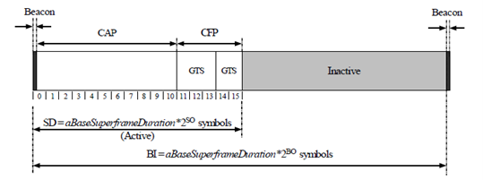
Figure-1: The IEEE 802.15.4 Frame Structure

When a transmitted packet collides or is corrupted by the PHY layer noise, the ACK packet is not generated which the transmitter interprets as packet delivery failure. The node reattempts the same packet for a maximum of a Max FrameRetries times before discarding it at the MAC layer. After transmitting a packet, the node turns to Rx-mode and waits for the ACK. The macAckWaitDuration determines the maximum amount of time a node must wait to receive the ACK before declaring that the packet (or the ACK) has collided. The default values of macminBE, macmaxBE, macMaxCSMABackoffs, and a Max FrameRetries are 3, 5, 4, and 3.

Objectives of the Experiment

In Section 6.1.2, we saw that the IEEE 802.15.4 PHY provides a bit rate of 250 Kbps, which has to be shared among the nodes sharing the 2 MHz channel on which this network runs. In the simulation experiment, the packets will have an effective length of 109 bytes (109 B = 872 bits). Thus, over a 250 Kbps link, the maximum packet transmission rate is \(\frac{250 \times 1000}{872} = 286.70\ \)packets per second. We notice, however, from the protocol description in Section 6.1.2, that due to the medium access control, before each packet is transmitted the nodes must contend for the transmission opportunity. This will reduce the actual packet transmission rate well below 286.7.

In this experiment, just one node will send packets to a receiver. Since there is no contention (there being only one transmitter) there is no need for medium access control, and packets could be sent back-to-back. However, the MAC protocol is always present, even with one node, and we would like to study the maximum possible rate at which a node can send back-to-back packets, when it is the only transmitter in the network. Evidently, since there is no uncertainty due to contention from other nodes, the overhead between the packets can be calculated from the protocol description in Section 6.1.2. This has been done in Section 6.1.6.

This analysis will provide the maximum possible rate at which a node can send packets over the IEEE 802.15.4 channel. Then in Section 6.1.7, we compare the throughput obtained from the simulation with that obtained from the analysis. In the simulation, in order to ensure that the node sends at the maximum possible rate, the packet queue at the transmitting node never empties out. This is ensured by inserting packets into the transmitting node queue at a rate higher than the node can possibly transmit.

NetSim Simulation Setup

Open NetSim and click on Experiments>IOT-WSN> One Hop IoT Network over IEEE 802.15.4 click on the tile in the middle panel to load the example as shown in below Figure-2.

Figure-2: List of scenarios for the example of One Hop IoT Network over IEEE 802.15.4

10s Simulation sample

NetSim UI displays the configuration file corresponding to this experiment as shown below Figure-3.

Figure-3: Network set up for studying the One Hop IoT Network over IEEE 802.15.4

Simulation Procedure

The following set of procedures were done to generate this sample:

Step 1: A network scenario is designed in NetSim GUI comprising of 2 Wireless Sensors, a LOWPAN Gateway, 1 Router, and 1 Wired Node from IoT library.

Step 2: In the Interface Zigbee > Data Link Layer of Wireless Sensor 1, Ack Request is set to Enable, and Max Frame Retries is set to 7. These settings will be automatically applied to Wireless Sensor 2 since the parameters are global. To configure these settings, click on the wireless sensor, expand the property panel on the right, and set the parameters as mentioned.

Step 3: In the Interface Zigbee > Data Link Layer of LOWPAN Gateway, Beacon Mode is set to Disable by default.

Step 4: Click on Ad hoc link and expand the link property panel on right and set channel characteristics to No pathloss.

Step 5: Configure Custom application between Sensor 1 to Wired node 5 by clicking on set traffic tab from ribbon on the top. Click on the created application, expand the application property panel on the right, and set the transport protocol to UDP, the packet size to 70 bytes, and the inter arrival time to 4000 µs.

The Packet Size and Inter Arrival Time parameters are set such that the Generation Rate equals 140 Kbps. Generation Rate can be calculated using the formula:

\[Generation\ Rate\ (Mbps)\ = \ Packet\ Size\ (Bytes)\ *\ 8/Interarrival\ time\ (µs)\]

NOTE: If the size of the packet at the Physical layer is greater than 127 bytes, the packet gets fragmented. Taking into account the various overheads added at different layers (which are mentioned below), the packet size at the application layer should be less than 80 bytes.

Step 6: Run simulation for 10 Seconds and note down the throughput.

Similarly, do the other samples by increasing the simulation time to 50, 100, and 200 Seconds respectively and note down the throughputs.

Analysis of Maximum Throughput

We have set the Application layer payload as 70 bytes in the Packet Size and when the packet reaches the Physical Layer, various other headers get added like Table-1.

App layer Payload	70 bytes
Transport Layer Header	8 bytes
Network Layer Header	20 bytes
MAC Header	5 bytes
PHY Header (includes Preamble, and Start Packet Delimiter)	6 bytes
Packet Size	109 bytes

Table-1: Overheads added to a packet as it flows down the network stack

By default, NetSim uses Unslotted CSMA/CA and so, the packet transmission happens after a Random Back Off, CCA, and Turn-Around-Time and is followed by Turn-Around-Time and ACK Packet and each of them occupies specific time set by the IEEE 802.15.4 standard as per the timing diagram shown below Figure-4.

Figure-4: Zigbee timing diagram

From IEEE standard, each slot has 20 Symbols in it and each symbol takes 16µs for transmission.

Symbol Time	\[\mathbf{T}_{\mathbf{s}}\]	16 µs
Slot Time	\[20 \times T_{s}\]	0.32 ms
Random Backoff Average	\(3.5\)*Slots	1.12 ms
CCA	\(0.4\)*Slots	0.128 ms
Turn-around-Time	\(0.6\)*Slots	0.192 ms
Packet Transmission Time	\(10.9\)*Slots	3.488 ms
Turn-around-Time	\(0.6\)*Slots	0.192 ms
ACK Packet Time	\(0.6\)*Slots	0.192 ms
Total Time	\(\mathbf{16.6}\)*Slots	5.312 ms

Table-2: Symbol times as per IEEE standard

\[Analytical\ Application\ Throughput\ = \ \frac{70(bytes)inApplayer*8}{5.312\ ms} = 105.42\ kbps\]

Comparison of Simulation and Calculation

Result Analysis	Throughput in
Throughput from simulation	104.74 kbps
Throughput from analysis	105.42 kbps

Table-3: Results comparison form simulation and theoretical analysis

Throughput from theoretical analysis matches the results of NetSim’s discrete event simulation. The slight difference in throughput is due to two facts that

• The average of random numbers generated for backoff need not be exactly 3.5 as the simulation is run for short time.

• In the packet trace one can notice that there are OSPF and AODV control packets (required for the route setup process) that sent over the network. The data transmissions occur only after the control packet transmissions are completed.

As we go on increasing the simulation time, the throughput value obtained from simulation approaches the theoretical value as can be seen from the table below Table-4.

Sample	Simulation Time (sec)	Throughput (kbps)
1	10	103.60
2	50	104.62
3	100	104.57
4	200	104.70

Table-4: Throughput comparison with different simulation times

IoT – Multi-Hop Sensor-Sink Path (Level 3)

NOTE: It is recommended to carry out this experiment in Standard Version of NetSim.

Introduction

The Internet provides the communication infrastructure for connecting computers, computing devices, and people. The Internet is itself an interconnection of a very large number of interconnected packet networks, all using the same packet networking protocol. The Internet of Things will be an extension of the Internet with sub-networks that will serve to connect “things” among themselves and with the larger Internet. For example, a farmer can deploy moisture sensors around the farm so that irrigation can be done only when necessary, thereby resulting in substantial water savings. Measurements from the sensors have to be communicated to a computer on the Internet, where inference and decision-making algorithms can advise the farmer as to required irrigation actions.

Farms could be very large, from a few acres to hundreds of acres. If the communication is entirely wireless, a moisture sensor might have to communicate with a sink that is 100s of meters away. As the distance between a transmitter and a receiver increase, the power of the signal received at the receiver decreases, eventually making it difficult for the signal processing algorithms at the receiver to decode the transmitted bits in the presence of the ever-present thermal noise. Also, for a large farm there would need to be many moisture sensors; many of them might transmit together, leading to collisions and interference.

Theory

The problem of increasing distance between the transmitter and the receiver is solved by placing packet routers between the sensors and the sink. There could even be multiple routers on the path from the sensor to the sink, the routers being placed so that any intermediate link is short enough to permit reliable communication (at the available power levels). We say that there is a multi-hop path from a sensor to the sink.

By introducing routers, we observe that we have a system with sensors, routers, and a sink; in general, there could be multiple sinks interconnected on a separate edge network. We note here that a sensor, on the path from another sensor to the sink, can also serve the role of a router. Nodes whose sole purpose is to forward packets might also need to be deployed.

The problem of collision and interference between multiple transmission is solved by overlaying the systems of sensors, routers, and sinks with a scheduler which determines (preferably in a distributed manner) which transmitters should transmit their packets to which of their receivers.

Figure-5: Data from Sensor A to Sink I takes the path A-B-D-I while data from sensor C to Sink I takes the path C-D-I

In this experiment, we will use NetSim Simulator to study the motivation for the introduction of packet routers, and to understand the performance issues that arise. We will understand the answers to questions such as:

1. How does packet error rate degrade as the sensor-sink distance increases?

2. How far can a sensor be from a sink before a router needs to be introduced?

3. A router will help to keep the signal-to-noise ratio at the desired levels, but is there any adverse implication of introducing a router?

Network Setup

Open NetSim and click on Experiments> IOT-WSN> IoT Multi Hop Sensor Sink Path > Packet Delivery Rate and Distance then click on the tile in the middle panel to load the example as shown in below Figure-6.

Figure-6: List of scenarios for the example of IoT Multi Hop Sensor Sink Path

Packet Delivery Rate vs. Distance

In this part, we perform a simulation to understand, “How the distance between the source and sink impacts the received signal strength (at the destination) and in turn the packet error rate?” We will assume a well-established path-loss model under which, as the distance varies, the received signal strength (in dBm) varies linearly. For a given transmit power (say 0dBm), at a certain reference distance (say 8m) the received power is \(c_{0}\)dBm and decreases beyond this point as \(- 10\eta\ \log_{10}{d\ }\ \) for a transmitter-receiver distance of \(d\). This is called a power-law path loss model, since in mW the power decreases as the \(\eta\) power of the distance \(d\). The value of \(\eta\) is 2 for free space path loss and varies from 2 to 5 in the case of outdoor or indoor propagation. Values of \(\eta\ \)are obtained by carrying out experimental propagation studies.

Distance vs BER PER and RSSI sample

NetSim UI displays the configuration file corresponding to this experiment as shown below Figure-7.

Figure-7: Network set up for studying the Distance vs BER PER and RSSI sample

Procedure

The following set of procedures were done to generate this sample:

Step 1: A network scenario is designed in the NetSim GUI comprising of a WSN Sink and 1 Wireless Sensor in Wireless Sensor Networks.

Note: NetSim currently supports a maximum of only one device, such as a WSN Sink.

Step 2: Set grid length as 150 x 200 from grid setting property panel on the right. This needs to be done before the any device is placed on the grid.

This grid length is initially configured for running a few samples, and as the distance between the sensor and the sink increases, the grid length is adjusted accordingly

Step 3: The distance between the WSN Sink and Wireless Sensor is 10 meters.

Step 4: In the Network Layer properties of Wireless Sensor 2, the Routing Protocol is set to AODV. To configure properties for any node, click on the node, expand the property panel on the right side, and adjust the settings as described in the following step.

Since the routing protocol is a global property, changing it on one node will affect the sink node as well.

Step 5: In the Interface Zigbee > Data Link Layer of Wireless Sensor 2, Ack Request is set to Enable and Max Frame Retries is set to 4. Similarly, the same settings are done in WSN Sink.

Step 6: In the Interface Zigbee > Physical Layer of Wireless Sensor 2, Transmitter Power is set to 0.5mW, Receiver Sensitivity is set to -105dBm, and ED Threshold is set to -115dBm.

Step 7: Click on link and expand property panel on the right and set the Channel characteristics: Path loss only; Path loss model: Log Distance; Path loss exponent: 3.7.

Step 8: Configure the CUSTOM application between the sensor and sink nodes by clicking on the 'Set Traffic' tab in the ribbon at the top. To set application properties, click on the created application, expand the application property panel on the right, and set the Transport Protocol to UDP, Packet Size to 70 bytes, and Inter Arrival Time to 4000 µs.

The Packet Size and Inter Arrival Time parameters are set such that the Generation Rate equals 140 Kbps. Generation Rate can be calculated using the formula:

\[Generation\ Rate\ (Mbps)\ = \ Packet\ Size\ (Bytes)\ *\ 8/Interarrival\ time\ (µs)\]

Step 9: The following procedures were followed to set Static IP:

Go to Network Layer properties of Wireless Sensor 2 Enable - Static IP Route ->Click on Configure Via UI.

Figure-8: Network layer properties window

Static IP Routing Dialogue box gets open.

Enter the Network Destination, Gateway, Subnet Mask, Metrics, and Interface ID. Click on Add.

You will find the entry added to the below Static IP Routing Table as shown below.

Click on OK.

Figure-9: Static Route Configuration Window

Step 9: IEEE 802.15.4 Radio Measurements log can be enabled by clicking on Configure Reports tab and Plots as shown below.

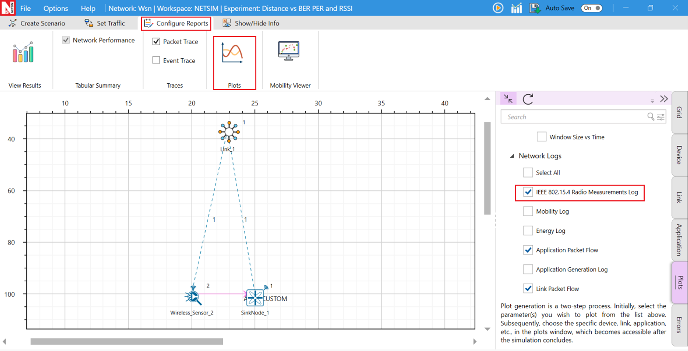
Figure-10: Enabling log files in NetSim GUI.

Step 10: Packet Trace is also enabled. At the end of the simulation, a very large .csv file is containing all the packet information is available for the users to perform packet level analysis.

Step 11: Enable the Application and Link plots and run the simulation for 10 seconds. Once the simulation is complete, open the IEEE 802.15.4 Radio Measurements log from the NetSim simulation results window.

Figure-11: Opening IEEE 802.15.4 Radio Measurements log from NetSim Simulation results window

In the IEEE 802.15.4 Radio Measurements log, filter the Control Packet Type to App1_CUSTOM and observe the Rx Power (RSSI) and BER values.

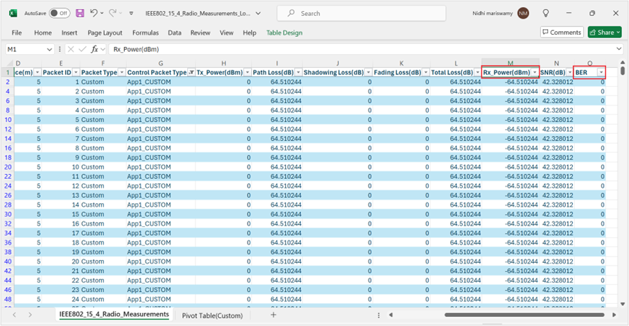
Figure-12: RSSI and BER values in IEEE 802.15.4 Radio Measurements log

Output for Distance vs BER PER and RSSI sample

RSSI, PER, BER vs. Distance (path-loss: linear in log-distance, with \(\mathbf{\eta = 3.7}\))
Distance(m)	RSSI (dBm) (Pathloss model)	BER	PER	PLR (After MAC retransmissions*)
10	-64.7	0	0	0
20	-75.84	0	0	0
30	-82.35	0	0	0
40	-86.98	0	0	0
50	-90.56	0	0	0
60	-93.49	0.000002	0.001742	0
70	-95.97	0.00024	0.1874	0
80	-98.11	0.00318	0.9376	0.621
90	-100.01	0.0141	0.999996	1
100	-101.7	0.03546	1	1
110	-103.64	0.07421	1	1
120	-104.63	0.09871	1	1

Table-5: Table showing RSSI, BER results obtained from IEEE 802.15.4 Radio Measurement log and calculated PER value.

Comparison Charts

(a)

(b)

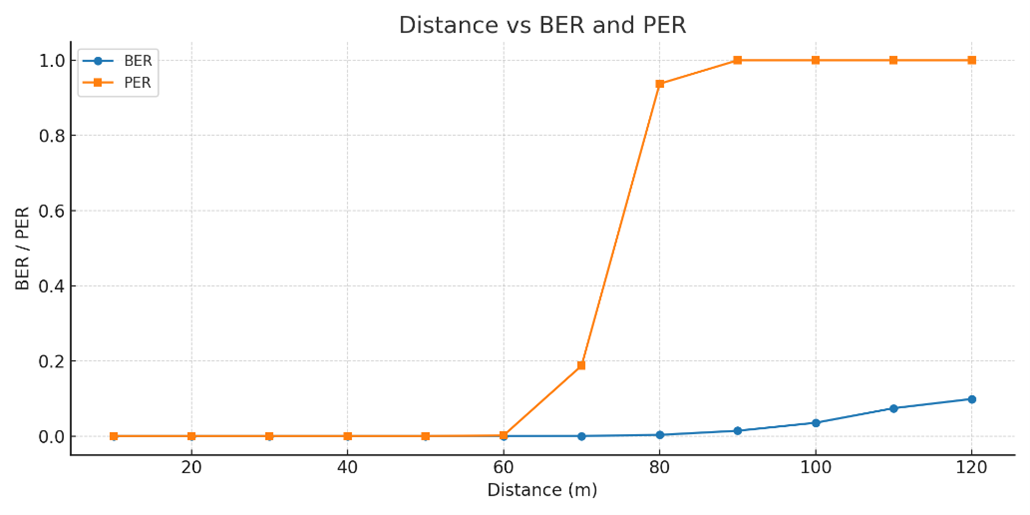
Figure-13: (a) Distance Vs. BER, PER and (b) Distance vs. RSSI

The IEEE 802.15.4 MAC implements a retransmission scheme that attempts to recover errored packets by retransmission. If all the retransmission attempts are also errored, the packet is lost.

The table above reports the RSSI (Received Signal Strength), BER (Bit Error Rate), and Packet Error Rate (PER), and the Packet Loss Rate (PLR) as the distance between the sensor to the sink is increased from 10m to 120m with path loss exponent \(\eta = 3.7\). We see that the BER is 0 until a received power of about -90dBm. At a distance of 60m the received power is -93 dBm, and we notice a small BER of \(2 \times 10^{- 6}\). As the distance is increased further the BER continues to grow and at 80m the BER is about \(0.00318\), yielding \(PER = 0.94,\) and \(PLR = \ 0.62.\ \) Here \(PER\ \) is obtained from the following formula (which assumes independent biterrors across a packet)

\[PER\ = \ 1 - (1 - BER)^{PL},\]

Where,

\[PL - \ packet\ length\ in\ bits\ at\ the\ PHY\ layer\]

\[PL\ (bits) = \left( 70\ (payload) + 39(overhead) \right)*8\]

The \(PLR\) in the above table has been obtained from NetSim, which implements the details of the IEEE 802.15.4 MAC acknowledgement and reattempt mechanism. This mechanism is complex, involving a MAC acknowledgement, time-outs, and multiple reattempts. Analysis of the \(PLR,\ \)therefore, is not straightforward. Assuming that the probability of MAC acknowledgement error is small (since it is a small packet), the \(PLR\ \)can be approximated as \(PER^{K + 1}\), where \(K\ \) is the maximum number of times a packet can be retransmitted.

\[PLR = \frac{Total\ number\ of\ Lost\ Packet\ }{Total\ number\ of\ Packet\ Sent\ by\ Source\ MAC}\]

\[Total\ number\ of\ Lost\ packets = \ Total\ number\ of\ Packet\ Sent\ by\ SourceMAC - Packets\ Received\ at\ Destination\ MAC\]

Steps to calculate Packet Loss Rate

• Open Packet Trace from the Results Dashboard. Filter the PACKET TYPE column as Custom and note down the packet id of the last packet sent from the PACKET ID column.

Figure-14: Packet Trace

This represents the total number of packets sent by the source.

• Note down the Packets Received from the Application Metrics in the Simulation results window as shown in Figure 6 15.

Figure-15: Application metrics table in Result Dashboard

This represents the total number of packets received at the destination.

• Calculate the total number of Lost Packets and PLR as follows:

For the above case,

\[\ Total\ number\ of\ Packet\ Sent\ by\ SourceMAC = 425\]

\[Packets\ Received\ at\ Destination\ MAC = 161\]

\[Total\ number\ of\ Lost\ packets = 425 - 161 = 264\]

\[PLR = \frac{264}{425} = 0.621\]

Inference

It is clear that Internet applications, such as banking and reliable file transfer, require that all the transmitted data is received with 100% accuracy. The Internet achieves this, in spite of unreliable communication media (no medium is 100% reliable) by various protocols above the network layer. Many IoT applications, however, can work with less than 100% packet delivery without affecting the application. Take, for example, the farm moisture sensing application mentioned in the introduction. The moisture levels vary slowly; if one measurement is lost, the next received measurement might suffice for the decision-making algorithm. This sort of thinking also permits the IoT applications to utilize cheap, low power devices, making the IoT concept practical and affordable.

With the above discussion in mind, let us say that the application under consideration requires a measurement delivery rate of at least \(80\%\). Examining the table above, we conclude that the sensor-sink distance must not be more than \(60\) meters. Thus, even a \(1\) acre farm \((61m \times 61m)\) would require multi-hopping to connect sensors to a sink at the edge of the farm.

In Part 2 of this experiment, we will study the placement of a single router between the sensor and the sink, to increase the sensor-sink distance beyond 60 meters.

Reaching a Longer Distance by Multihopping

Direct sensor sink link sample

NetSim UI displays the configuration file corresponding to this experiment as shown below Figure-16.

Figure-16: Network set up for studying the Direct sensor sink link sample

Procedure

The following changes in settings are done from the previous sample:

Step 1: The distance between the WSN Sink and Wireless Sensor is 40 meters.

Step 2: In the Interface Zigbee > Data Link Layer of Wireless Sensor 2, Ack Request is set to Enable and Max Frame Retries is set to 3. To configure properties for any node, click on the node, expand the property panel on the right side, and adjust the settings as described.

Step 3: The Ad hoc Link properties are set as follows Figure-17.

Figure-17: Wireless Link properties

Step 4: Configure the CUSTOM application between the sensor and sink nodes by clicking on the 'Set Traffic' tab in the ribbon at the top. To set application properties, click on the created application, expand the application property panel on the right, and set the Transport Protocol to UDP, Packet Size to 70 bytes, and Inter Arrival Time to 100000 µs.

The Packet Size and Inter Arrival Time parameters are set such that the Generation Rate equals 5.6 Kbps. Generation Rate can be calculated using the formula:

\[Generation\ Rate\ (Mbps)\ = \ Packet\ Size\ (Bytes)\ *\ 8/Interarrival\ time\ (µs)\]

Step 5: Run the Simulation for 100 Seconds. Once the simulation is complete, note down the Packet Generated, Packet Received and Throughput values from the Application Metrics.

Note down the Packet Errored and Packet Collided from the Link Metrics.

Figure-18: NetSim Results window displaying the number of received, collided, and errored packets.

Router between sensor and sink sample

NetSim UI displays the configuration file corresponding to this experiment as shown below Figure-19.

Figure-19: Network set up for studying the Router between sensor and sink sample

Procedure

The following changes in settings are done from the previous sample:

Step 1: One more Wireless Sensor is added to this network. The distance between Wireless Sensor 2 and Wireless Sensor 3 is 60 meters and the distance between Wireless Sensor 3 and the WSN Sink is 60 meters.

Step 2: The following procedures were followed to set Static IP:

In Network Layer properties of Wireless Sensor 2 Enable - Static IP Route ->Click on Configure via UI as shown in Figure-20.

Figure-20: Network layer properties window

Static IP Routing Dialogue box gets open.

Enter the Network Destination, Gateway, Subnet Mask, Metrics, and Interface ID. Click on Add.

You will find the entry added to the Static IP Routing Table as shown below. Similarly, Static IP is set for Wireless Sensor 3 as shown below Figure-21.

Figure-21: Static Route configuration for Wireless Sensor 3

Step 3: Run the Simulation for 100 Seconds. Once the simulation is complete, note down the Packet Generated, Packet Received and Throughput values from the Application Metrics.

Note down the Packet Errored and Packet Collided from the Link Metrics as shown in Table-6

Figure-22: NetSim Results window displaying the number of received, collided, and errored packets.

Output for Router between sensor and sink sample

	Source-Sink Distance(m)	Packets Generated	Packets Received	Packets Errored (PHY)	Packets Collided	Packet Loss (MAC)	PLR	Mean Delay \(\mathbf{(\mu s)}\)
Direct sensor-sink link	60	1000	1000	243	0	0	0	6440.74
Router between sensor and sink	120 (router at midpoint)	1000	1007	537	0	-7	-0.007	14180.93

Table-6: Packet Generated/Received/Errored/Collided and Mean delay from result dashboard

NOTE: Packet loss (PHY) is the number of packets that were received in error and then recovered by retransmission. Packets received is slightly higher than packets generated on account of retransmissions of successful packets in case of ACK errors.

Inference

In Distance vs BER PER and RSSI sample of this experiment, we learnt that if the sensor device uses a transmit power of -3dBm (0.5mW), then for one-hop communication to the sink, the sensor-sink distance cannot exceed 60m. If the sensor-sink distance needs to exceed 60m (see the example discussed earlier), there are two options:

1. The transmit power can be increased. There is, however, a maximum transmit power for a given device. Wireless transceivers based on the CC 2420 have a maximum power of 0dBm (i.e., about 1 mW), whereas the CC 2520 IEEE 802.15.4 transceiver provides maximum transmit power of 5dBm (i.e., about 3 mW). Thus, given that there is always a maximum transmit power, there will always be a limit on the maximum sensor-sink distance.

2. Routers can be introduced between the sensor and the sink, so that packets from the sensor to the sink follow a multihop path. A router is a device that will have the same transceiver as a sensor, but its microcontroller will run a program that will allow it to forward packets that it receives. Note that a sensor device can also be programmed to serve as a router. Thus, in IOT networks, sensor devices themselves serve as routers.

In this part of the experiment, we study the option of introducing a router between a sensor and the sink to increase the sensor-sink distance. We will compare the performance of two networks, one with the sensor communicating with a sink at the distance of 60m, and another with the sensor-sink distance being 120m, with a sensor at the mid-point between the sensor and the sink.

Direct sensor sink link sample simulates a one hop network with a sensor-sink distance of 60m. We recall from Part 1 that, with the transceiver model implemented in NetSim, 60m is the longest one hop distance possible for 100% packet delivery rate. In Router between sensor and sink sample, to study the usefulness of routing we will set up network with a sensor-sink distance of 120m with a packet router at the midpoint between the sensor and the sink.

The measurement process at the sensor is such that one measurement (i.e., one packet) is generated every 100ms. The objective is to deliver these measurements to the sink with 100% delivery probability. From Part 1 of this experiment, we know that a single hop of 90m will not provide the desired packet delivery performance.

The Table at the beginning of this section shows the results. We see that both networks are able to provide a packet delivery probability of 100%. It is clear, however, that since the second network has two hops, each packet needs to be transmitted twice, hence the mean delay between a measurement being generated and it being received at the sink is doubled. Thus, the longer sensor-sink distance is being achieved, for the same delivery rate, at an increased delivery delay.

The following points may be noted from the table:

1. The number of packets lost due to PHY errors. The packet delivery rate is 100% despite these losses since the MAC layer re-transmission mechanism is able to recover all lost packets.

2. There are no collisions. Since both the links (sensor-router and router-sink) use the same channel and there is no co-ordination between them, it is possible, in general for sensor-router and router-sink transmissions to collide. This is probable when the measurement rate is large, leading to simultaneously nonempty queues at the sensor and router. In this experiment we kept the measurement rate small such that the sensor queue is empty when the router is transmitting and vice versa. This avoids any collisions.

Performance Evaluation of a Star Topology IoT Network (Level 3)

Introduction

In IOT experiments 20 and 21 we studied a single IoT device connected to a sink (either directly or via IEEE 802.15.4 routers). Such a situation would arise in practice, when, for example, in a large campus, a ground level water reservoir has a water level sensor, and this sensor is connected wirelessly to the campus wireline network. Emerging IoT applications will require several devices, in close proximity, all making measurements on a physical system (e.g., a civil structure, or an industrial machine). All the measurements would need to be sent to a computer connected to the infrastructure for analysis and inferencing. With such a scenario in mind, in this experiment, we will study the performance of several IEEE 802.15.4 devices each connected by a single wireless link to a sink. This would be called a “star topology” as the sensors can be seen as the spikes of a “star.”

We will set up the experiment such that every sensor can sense the transmissions from any other sensor to the sink. Since there is only one receiver, only one successful transmission can take place at any time. The IEEE 802.15.4 CSMA/CA multiple access control will take care of the coordination between the sensor transmissions. In this setting, we will conduct a saturation throughput analysis. The IoT communication buffers of the IEEE 802.15.4 devices will always be nonempty, so that as soon as a packet is transmitted, another packet is ready to be sent. This will provide an understanding of how the network performs under very heavy loading. For this scenario we will compare results from NetSim simulations against mathematical analyses.

Details of the IEEE 802.15.4 PHY and MAC have been provided in the earlier IOT experiments 20 and 21, and their understanding must be reviewed before proceeding further with this experiment. In this experiment, all packets are transferred in a single hop from and IoT device to the sink. Hence, there are no routers, and no routing to be defined.

NetSim Simulation Setup

Open NetSim and click on Experiments> IOT-WSN> IOT Star Topology then click on the tile in the middle panel to load the example as shown in below Figure-23.

Figure-23: List of scenarios for the example of IOT Star Topology

The simulation scenario consists of n nodes distributed uniformly around a sink (PAN coordinator) at the center. In NetSim the nodes associate with the PAN coordinator at the start of the simulation. CBR traffic is initiated simultaneously from all the nodes. The CBR packet size is kept as 10 bytes to which 20 bytes of IP header, 7 bytes of MAC header and 6 bytes of PHY header are added. To ensure saturation, the CBR traffic interval is kept very small; each node’s buffer receives packets at intervals of 5 ms.

Procedure

Sensor-1

NetSim UI displays the configuration file corresponding to this experiment as shown below Figure-24.

Figure-24: Network set up for studying the Sensor 1

The following set of procedures were done to generate this sample:

Step 1: A network scenario is designed in NetSim GUI comprising of 1 SinkNode, and 1 wireless sensor in the “WSN” Network Library.

Step 2: Click on sensor, expand the property panel on right and configure the static route in network layer as shown in below Table-7.

Network Destination	Gateway	SubnetMask	Metrics	Interface ID
192.168.0.0	192.168.0.1	255.255.255.0	1	1

Table-7: Static route for Wireless sensor

Step 3: Click on Adhoc link, expand the link property panel on right and set channel characteristics to No pathloss.

Step 4: Configure a CBR application from Wireless Sensor 2 (Source) to Sink Node 1 (Destination) by clicking on the Set Traffic tab in the ribbon at the top. Then, click on the created application and set the packet size to 10 bytes, the inter arrival time to 5000 µs, the start time to 5 seconds, and the transport protocol to UDP.

Step 5: Plots are enabled from configure reports tab and Simulation time is set to 100 seconds.

Increase wireless sensor count to 2, 3, and 4 with the same above properties to design Sensor-2, 3, and 4.

Sensor-5: NetSim UI displays the configuration file corresponding to this experiment as shown below Figure-25.

Figure-25: Network set up for studying the Sensor-5

The following set of procedures were done to generate this sample:

Step 1: Click on sensor, expand the property panel on right and configure the static route in network layer as shown in below Table-8.

Network Destination	Gateway	SubnetMask	Metrics	Interface ID
192.168.0.0	192.168.0.1	255.255.255.0	1	1

Table-8: Static route for Wireless sensors

Step 2: Configure CBR application by clicking on set traffic tab from the ribbon on the top. Set the applications properties as mentioned in below Table-9.

	App 1	App 2	App 3	App 4	App 5
Application	CBR	CBR	CBR	CBR	CBR
Source ID	2	3	4	5	6
Destination ID	1	1	1	1	1
Start time	5s	5s	5s	5s	5s
Transport protocol	UDP	UDP	UDP	UDP	UDP
Packet Size	10bytes	10bytes	10bytes	10bytes	10bytes
Inter-Arrival Time	5000 μs	5000 μs	5000 μs	5000 μs	5000 μs

Table-9: Detailed Application properties

Step 3: Plots are enabled in NetSim GUI. Click on Run simulation. The simulation time is set to 100 seconds.

Increase wireless sensor count to 10, 15, 20, 25, 30, 35, 40, and 45 with the same above properties to design Sensor-6, 7, 8, 9, 10, 11, 12, and 13.

Output

The aggregate throughput of the system can be got by adding up the individual throughput of the applications. NetSim outputs the results in units of kilobits per second (kbps). Since the packet size is 80 bits we convert per the formula

\[Aggregate\ Throughput\ (pkts\ per\ sec) = \frac{Aggregate\ Throughput\ (kbps)*1000}{80}\]

Number of Nodes	Aggregate Throughput (Kbps)	Aggregate Throughput (pkts/s)
1	16.00	200.00
2	23.07	288.38
3	22.67	283.38
4	22.33	279.13
5	21.85	273.13
10	18.60	232.50
15	15.26	190.75
20	12.32	154.00
25	9.98	124.75
30	7.84	98.00
35	6.17	77.13
40	4.88	61.00
45	3.72	46.50

Table-10: Aggregate throughput for Star topology scenario

Figure-26: The plot illustrates the relationship between aggregate throughput (measured in packets per second) and the number of nodes within an IoT star topology network. It demonstrates how throughput varies as the network size increases

Discussion

In Figure-26 we plot the throughput in packets per second versus the number of IoT devices in the star topology network. We make the following observations:

1. Notice that the throughput for a single saturated node is 200 packets per second, which is just the single hop throughput from a single saturated node, when the packet payload is 10 bytes. When a node is by itself, even though there is no contention, still the node goes through a backoff after every transmission. This backoff is a waste and ends up lowering the throughput as compared to if the node knew it was the only one in the network and sent packets back-to-back.

2. When there are two nodes, the total throughput increases to 287.5 packets per second. This might look anomalous. In a contention network, how can the throughput increase with more nodes? The reason can be found in the discussion of the previous observation. Adding another node helps fill up the time wasted due to redundant backoffs, thereby increasing throughput.

3. Adding yet another node results in the throughput dropping to 282.5 packets per second, as the advantage gained with 2 nodes (as compared to 1 node) is lost due to more collisions.

4. From there on as the number of nodes increases the throughput drops rapidly to about 100 packets per second for about 30 nodes.

5. The above behaviour must be compared with a Experiment 12 where several IEEE 802.11 STAs, with saturated queues, were transmitting packets to an AP. The throughput increased from 1 STA to 2 STAs, dropped a little as the number of STAs increased and then flattened out. On the other hand, in IEEE 802.15.4 the throughput drops rapidly with increasing number of STAs. Both IEEE 802.11 and IEEE 802.15.4 have CSMA/CA MACs. However, the adaptation in IEEE 802.11 results in rapid reduction in per-node attempt rate, thus limiting the drop in throughput due to high collisions. On the other hand, in IEEE 802.15.4, the per-node attempt rate flattens out as the number of nodes is increased, leading to high collisions, and lower throughput. We note, however, that IoT networks essentially gather measurements from the sensor nodes, and the measurement rates in most applications are quite small.

References

1. Chandramani Kishore Singh, Anurag Kumar. P. M. Ameer (2007). Performance evaluation of an IEEE 802.15.4 sensor network with a star topology. Wireless Network (2008) 14:543

Study the 802.15.4 Superframe Structure and analyze the effect of Superframe order on throughput (Level 3)

Introduction

A coordinator in a PAN can optionally bound its channel time using a Superframe structure which is bound by beacon frames and can have an active portion and an inactive portion. The coordinator enters a low-power (sleep) mode during the inactive portion.

The structure of this Superframe is described by the values of macBeaconOrder and macSuperframeOrder. The MAC PIB attribute macBeaconOrder, describes the interval at which the coordinator shall transmit its beacon frames. The value of macBeaconOrder, BO, and the beacon interval, BI, are related as follows:

For 0 ≤ BO ≤ 14, BI = aBaseSuperframeDuration * 2^BO symbols.

If BO = 15, the coordinator shall not transmit beacon frames except when requested to do so, such as on receipt of a beacon request command. The value of macSuperframeOrder, SO shall be ignored if BO = 15.

An example of a Superframe structure is shown in following Figure-27.

Figure-27: An example of the Super Frame structure

Theoretical Analysis

From the above Superframe structure,

\[Beacon\ Interval\ \ \ \ \ \ \ \ \ \ = \ aBaseSuperframeDuration*2^{BO}\]

\[Active\ part\ of\ SuperFrame\ = \ aBaseSuperframeDuration*2^{SO}\]

\[Inactive\ part\ of\ SuperFrame\ = \ aBaseSuperframeDuration*{(2}^{BO} - 2^{SO})\]

If Superframe Order (SO) is same as Beacon Order (BO) then there will be no inactive period and the entire Superframe can be used for packet transmissions.

If BO=10, SO=9 half of the Superframe is inactive and so only half of Superframe duration is available for packet transmission. If BO=10, SO=8 then (3/4)^th of the Superframe is inactive and so nodes have only (1/4)^th of the Superframe time for transmitting packets and so we expect throughput to approximately drop by half of the throughput obtained when SO=9.

Percentage of inactive and active periods in Superframe for different Superframe Orders is given below Table-11. This can be understood from Beacon Time Analysis section of the IoT-WSN technology library manual.

Beacon Order (BO)	Super Frame Order (SO)	Active part of Superframe(%)	Inactive part of Superframe (%)	Throughput estimated (%)
10	10	100	0	> 200% of T
10	9	50	50	Say T = 21.07 (Got from simulation)
10	8	25	75	50 % T
10	7	12.5	87.5	25 % T
10	6	6.25	93.75	12.5 % of T
10	5	3.125	96.875	6.25 % of T
10	4	1.5625	98.4375	3.12% of T
10	3	0.78125	99.21875	1.56 % of T

Table-11: Inactive and active periods in Superframe for different Superframe

We expect throughput to vary in the active part of the Superframe as sensors can transmit a packet only in the active portion.

Network Setup

Open NetSim and click on Experiments> IOT-WSN> 802.15.4 Superframe and effect of Superframe order on throughput then click on the tile in the middle panel to load the example as shown in below Figure-28.

Figure-28: List of scenarios for the example of 802.15.4 Superframe and effect of Superframe order on throughput

Super Frame Order 10 Sample

NetSim UI displays the configuration file corresponding to this experiment as shown below Figure-29.

Figure-29: Network set up for studying the Super Frame Order 10 Sample

Procedure

The following set of procedures were done to generate this sample:

Step 1: A network scenario is designed in NetSim GUI comprising of 2 Wireless Sensors and a WSN Sink in the “Wireless Sensor Networks” Network Library.

Step 2: Before we designed this network, in the Fast Config Window containing inputs for Grid Settings and Placement Strategy, the Grid Length and width were set to 500 and 250 meters respectively.

Step 3: Click on the WSN Sink, expand the property panel on the right, and set the Beacon mode to Enable. In the Data Link Layer of the Interface Zigbee, set the Beacon Order and Superframe Order to 10 as shown below.

Figure-30: Setting Superframe and Beacon order in Sink node

Step 4: The Ad hoc Link is used to link the Sensors and the WSN Sink in an ad hoc basis. To set the channel characteristics, click on Ad hoc link and expand link property panel on right and set channel characteristics to No pathloss.

Step 5: Configure a custom application between sensors by clicking on the 'Set Traffic' tab in the ribbon at the top. Click on the created application, set the packet size to 25 bytes, and set the inter-arrival time to 3000 µs.

The Packet Size and Inter Arrival Time parameters are set such that the Generation Rate approximately equals 67 Kbps. Generation Rate can be calculated using the formula:

\[Generation\ Rate\ (Mbps)\ = \ Packet\ Size\ (Bytes)\ *\ 8/Interarrival\ time\ (µs)\]

Step 6: Run the Simulation for 30 Seconds and note down the Throughput value.

Similarly, run the other samples by varying the Super Frame Order to 9, 8, 7, 6, 5, and 4 and note down the throughput values.

Output

The following are the throughputs obtained from the simulation for different Super Frame Orders Table-12.

Super Frame Order	Throughput (Kbps)	Theoretical Throughput (Kbps)
10	41.68	> 200% of T (T=21.07)
9	21.07	100 % T
8	10.5	50 % T
7	5.25	25 % T
6	2.63	12.5 % of T
5	1.30	6.25 % of T
4	0.62	3.12% of T

Table-12: Different Super Frame Orders vs. throughputs

To obtain throughput from simulation, payload transmitted values will be obtained from Link metrics and calculated using following formula:

\[Application\ Throughput(in\ Mbps) = \frac{Total\ payload\ delivered\ to\ destination\ (bytes)\ *\ 8}{Simulation\ Time(Millisecond)\ - App\ Start\ Time(Millisecond)}\]

Figure-31: This plot presents a comparative analysis of Superframe order against both simulated and theoretical throughput values. Simulation results agree well with theoretical expectations.

Comparison Chart: All the above plots highly depend upon the placement of Sensor in the simulation environment. So, note that even if the placement is slightly different the same set of values will not be got but one would notice a similar trend.

Inference

From the comparison chart both the simulation and theoretical throughputs match except for the case with no inactive period. A sensor will be idle if the last packet in its queue is transmitted. If a packet is generated in inactive period, then the packet has to wait in the queue till the next Superframe so sensor has packets waiting in its queue and so it cannot be idle in the next Superframe, but if there is no inactive period then there might be no packets waiting in the queue and so sensor can be idle resulting in lesser throughput.