← Back

Mobile Ad hoc Networks

Connectivity of a randomly deployed 1-D ad hoc network (Level 2)

Objective

To analyze the probability of connectivity of a randomly deployed 1-dimensional ad hoc network.

In the first part of the experiment, we analyze connectivity for a simple 2-node network. In the advanced section, we extend this analysis to \(n\) nodes.

Preliminaries

An important feature of wireless networks is that the node locations in a network are random, because of either mobility or deployment constraints. Thus, in exploring the fundamental performance limits of wireless networks, it is reasonable to model the node locations as random variables.

A network graph captures the communication capabilities among the nodes in the network and connectivity is an important network graph property. For a wireless network, the network graph also captures the communication constraints; for example, it can be used to specify the nodes that are in communication range of any node.

We assume that a transmission from node \(i\), located at \(X_{i}\), can be decoded at node\(\ j\), located at \(X_{j}\), if the Euclidean distance between \(X_{i}\) and \(X_{j}\) is less than \(r\) i.e., \(\left| X_{2} - X_{1} \right|, \leq r\) in 1-D , or \(\sqrt{{\left( Y_{2} - Y_{1} \right)^{2} + \left( X_{2} - X_{1} \right)}^{2}} \leq r\), in 2-D.

Mathematical analysis of a 2-node 1-D network

Consider a two-node, one-dimensional network with the location of each node uniformly distributed in \(\lbrack 0,\ z\rbrack\ \)and chosen independently of each other. Let the transmission range of both nodes be \(r\). We now obtain the probability that the two nodes are connected. Without loss of generality, let \(X_{1}\) be the location of the left node and \(X_{2}\) that of the right node; that is, \(X_{1} \leq X_{2}\). The two-node network is connected if \(X_{2}\ - \ X_{1}\ \leq \ r\). This is graphically shown in Figure-1. The set of values that \((X_{1},\ X_{2})\) can take is denoted by the area OAB. The set of \((X_{1},\ X_{2})\) that would result in a connected network is given by the shaded area S in the below figure.

Figure-1: S represents the feasible region of a random, connected 2-node, 1-dimensional ad hoc network.

S is the region satisfying \(X_{1}\ < \ X_{2}\) (by definition of \(X_{1}\) and \(X_{2}\)) and \(X_{2}\ - \ X_{1}\ \leq \ r\) (the connectivity requirement). Since the nodes are distributed uniformly in \(\lbrack 0,\ z\rbrack,\) the probability that the network is connected is the ratio of the area of S to the area of OAB. The area of S is\(\frac{z^{2}}{2} - \frac{(z - r)}{2}^{2}\)and that of OAB is \(\frac{z^{2}}{2}\). Thus, the probability that the network is connected is

\[P_{c} = 2 \cdot \left( \frac{r}{z} \right) - \left( \frac{r}{z} \right)^{2}\]

where, \(P_{c}\) is the network connectivity fraction or the probability of network connectivity, and

\(\frac{r}{z}\) is the normalized transmission range.

Modelling the transmission range

NetSim supports are wide range of pathloss models. In this experiment, we need to use a pathloss model whereby the transmission range of a node is r. This can be modelled using the Range based pathloss model in NetSim. In this model, the propagation loss depends only on the distance (range) between transmitter and receiver. There is a single Range attribute that determines the path loss. Receivers located at or within ‘Range’ see a 0 dB pathloss. Hence received power equals transmit power. Receivers beyond ‘Range’ see a 1000 dB pathloss. Hence received power will be close to -1000 dBm which is essentially zero in linear units.

Procedure to simulate this scenario in NetSim

1. In NetSim home window click on MANET section. Under the Grid settings, set Grid Width as 1000m and Grid length as 500m and under device placement strategy select Manually via Click and Drop.

Figure-2: Select the ‘Manually via click and drop’ option in grid setting window.

2. Deploy two wireless nodes. Set the mobility of both devices to No mobility, and position both wireless nodes at Y coordinate 250. The X coordinate can be any value at this stage. Since the X coordinate is a variable for this experiment, the exact setting is explained subsequently.

Figure-3: Set mobility model as No mobility

3. Configure a CBR application to communicate between the wireless nodes. Let the packet size be default, set the start time as 0 and Inter Arrival Time as 600,000.

Figure-4: Set IAT in application settings

4. Set Channel Characteristics as pathloss and Path Loss Model as Range based. The range (m) can be any value currently. This is another variable in this experiment and the exact settings are explained subsequently.

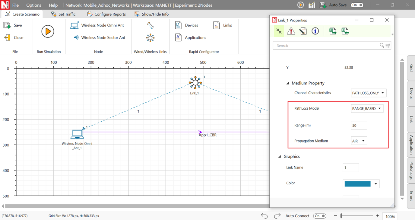
Figure-5: Channel characteristics properties

5. Add Static Route from Wireless Node 1 to Wireless Node 2. In Wireless Node 1 property, go to Network layer and make Static IP Route enable, then click on via GUI. The static routing setup neglects guiding control packets around it and doesn't account for RTS/CTS thresholds. This approach might disrupt data flow and affect collision management during data transmission in the network.

Figure-6: Enabling static route in wireless node 1.

• In the Static IP Routing Configuration Window, add destination IP address (enable Device IP in Show/Hide Info), gateway, subnet mask, metrics, interface id and click on Add.

Figure-7: Static Route Configuration

6. Save this scenario and open the experiment in the file explorer and open Configuration.netsim in Visual Studio.

Figure-8: Opening saved file location from ‘Your Work’ window

7. Within the POS 3D tag of both wireless nodes, replace the current X coordinates with a variable {n}, where n = 0, 1, 2, 3, and so on, representing an input variable from the multi-parameter sweeper. Similar procedure is repeated for pathloss Range. Set the simulation time as 0.5.

Figure-9: input variables for Multi-Parameter Sweeper

8. Save the configuration file and rename it as input.xml.

9. Download the multi-parameter sweeper from the given link https://github.com/NetSim-TETCOS/Connectivity-of-1D-ad-hoc-Networkv14.4/archive/refs/heads/main.zip

10. Paste input.xml and Config support folder into the 2Nodes folder.

11. Change the NetSim Path (line #2) to the current workspace bin_x64 path.

Figure-10: MultiParameterSweeper.py opened in the Visual Studio editor window.

12. Run MultiParameterSweeper.py using command prompt.

13. The multi-parameter sweeper runs 2000 simulations, varying X-coordinates between nodes and all transmission range values. It generates an output file named "result.csv" to store the collected data.

Procedure to obtain the number of time network is connected from results.

1. Open the results.csv file and in the toolbar's insert section, insert a table to the current section.

Figure-11: Opening Results.csv file

2. In the toolbar's insert section, insert a pivot table for the current table.

Figure-12: Inserting Pivot Table

3. In the pivot table add Range in Rows and Packets Received in Filters and Values. In the multi-parameter-sweeper, one packet is sent per simulation. A successful transmission is when the received packet is marked as 1, and unsuccessful if marked as 0. After creating the pivot table, it reflects the total occurrences of successful transmissions per range by summing up the received packets.

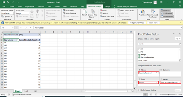
Figure-13: Pivot table settings

Simulation Results

Use the result.csv file to get the successful transmission probability table and its plot. From the principles of Monte Carlo simulations, the fraction of times the network is connected (from simulations) is nothing but the probability of network connectivity (from theory).

In the following table, the sum of packets obtained from the above pivot table is nothing but the count of times network is connected. The probability of network connectivity (analysis) is obtained using the formula \(P_{c} = 2 \cdot \left( \frac{r}{z} \right) - \left( \frac{r}{z} \right)^{2}\)

Transmission Range \(\mathbf{(r)}\) [m]	Normalized transmission range \(\mathbf{(r/z)\ }\)where \(\mathbf{z = 1000}\) [m]	Count of times network is connected (Total of 100 runs)	Network connectivity fraction (simulation)	Probability of network connectivity (analysis)
50	0.05	9	0.09	0.097
100	0.10	16	0.16	0.190
150	0.15	23	0.23	0.277
200	0.20	34	0.34	0.360
250	0.25	42	0.42	0.437
300	0.30	47	0.47	0.510
350	0.35	56	0.56	0.577
400	0.40	63	0.63	0.640
450	0.45	68	0.68	0.697
500	0.50	73	0.73	0.750
550	0.55	78	0.78	0.797
600	0.60	85	0.85	0.840
650	0.65	87	0.87	0.877
700	0.70	88	0.88	0.910
750	0.75	94	0.94	0.937
800	0.80	95	0.95	0.960
850	0.85	99	0.99	0.977
900	0.90	100	1.00	0.990
950	0.95	100	1.00	0.997
1000	1.00	100	1.00	1.000

Table-1: Results of NetSim simulation and analysis.

Figure-14: Plot comparing simulation results against analytical model for probability of network connectivity for different normalized transmission range values.

Advanced Topic: End-to-end connectivity of a network with n Nodes

Let there be \(n\) nodes in the network and let the location of node \(i\) be denoted by \(X_{i}\). \(X_{i}\ \)are i.i.d. with uniform distribution in \(\lbrack 0,\ z\rbrack\). Thus, the random network is represented by a random vector \(X\ = \ \left\lbrack X_{1},X_{2},\ .\ .\ .\ ,X_{n} \right\rbrack.\) Let \(p_{c}(n,\ z,\ r)\) be the probability that X represents a connected network when each node has a transmission range of r. Let \(\widehat{X} = \left\lbrack {\widehat{X}}_{1},\ {\ \widehat{X}}_{2},\ \ldots\ldots..\ {\widehat{X}}_{n} \right\rbrack\) be the node locations ordered according to their positions on \(\lbrack 0,z\rbrack\); that is, \(\ {\widehat{X}}_{1} < \ {\widehat{X}}_{2} < \ \ {\widehat{X}}_{3} < ...\ < \ {\widehat{X}}_{n}\). Define \(\ {\widehat{X}}_{0} = 0\). The condition \({\widehat{X}}_{i + 1} - \ \ {\widehat{X}}_{i} < \ r\) for \(i\ = \ 1,\ .\ .\ .\ ,\ (n\ - \ 1)\) needs to be satisfied for X to represent a connected network.

The derivation of the closed form analytical equation for \(p_{c}(n,\ z,\ r)\) is provided in pages 299 – 301 of [6]. It finally turns out that the probability that the network is connected it

\[p_{c}(n,\ z,\ r) = \ \frac{U_{c}(n,\ z,\ r)}{U(n,\ z)} = \ \sum_{k = 0}^{n - 1}\binom{n - 1}{k}( - 1)^{k}\frac{(z - kr)^{n}}{z^{n}}u(z - kr)\]

where \(u(z)\) is the unit step function i.e., \(u(z) = 0\) when \(z \leq 0\) and \(u(z) = 1\) when \(z > 0\).

Procedure to simulate the n node 1-D scenarios in NetSim

We conduct simulation experiments in NetSim for n= 5,10, and 20, and the procedure for 5-nodes is explained below. Follow similar steps for n=10, and 20.

1. In NetSim home window click on MANET section. Under the Grid settings, set Grid Length as 1000 and under device placement strategy select Manually via Click and Drop.

Figure-15: Select the ‘Manually via click and drop’ option in grid setting window.

2. Deploy five wireless nodes. Set the mobility of all five devices to NO MOBILITY, and position of all five wireless nodes at Y coordinate 250.

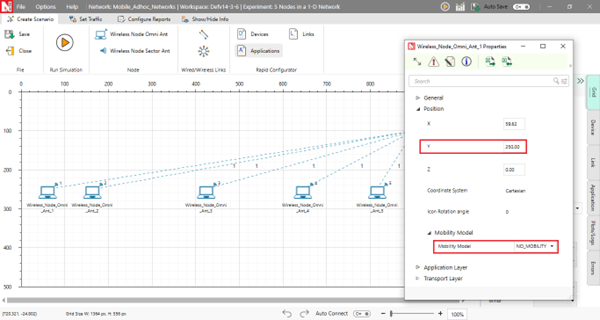
Figure-16: Device Placement and Mobility Settings

3. Configure a CBR application to communicate between the wireless nodes from Wireless node 1 to wireless node N, i.e node 1 to node 5. Let the packet size be default, set the start time as 0 and Inter Arrival Time as 600,000.

Figure-17: Set IAT in Application Settings

4. Set Channel characteristics as Pathloss and Pathloss model as Range based.

Figure-18: Set channel characteristics properties.

5. Add Static route from wireless node 1 to Wireless Node 5. The static routing setup neglects guiding control packets around it and doesn't account for RTS/CTS thresholds. This approach might disrupt data flow and affect collision management during data transmission in the network. In Wireless Node 1 properties, go to Network layer and make Static IP route enable, then click on via GUI.

Figure-19: Network Layer Settings

In the Static IP Routing Configuration Window, add destination IP address (it should be to the next Wireless Node i.e., 1>2, 2>3, … and so on), gateway, subnet mask, metrics, interface id. Click on Add to add the static route.

Figure-20: Static IP Routing Configuration Window

Wireless Node	Network Destination	Subnet Mask	Gateway	Metrics	Interface
Wireless Node 1	192.168.0.6	255.255.255.255	192.168.0.3	1	1
Wireless Node 2	192.168.0.6	255.255.255.255	192.168.0.4	1	1
Wireless Node 3	192.168.0.6	255.255.255.255	192.168.0.5	1	1
Wireless Node 4	192.168.0.6	255.255.255.255	192.168.0.6	1	1

Table-2: Static route configurations for wireless nodes.

6. Save this scenario and open the experiment in the file explorer and open Configuration.netsim in Visual Studio.

Figure-21: Your Work window

7. Within the POS 3D tag of all the wireless nodes, replace the current X coordinates with a variable {n}, where n = 0, 1, 2, 3, and so on, representing an input variable from the multi-parameter sweeper. Similar procedure is repeated for Pathloss range. Set the simulation time as 0.5.

Figure-22: Configuration file changes for Multi-Parameter Sweeper

8. Save the configuration file and rename it as input.xml.

9. Download the multi-parameter sweeper from the given link https://github.com/NetSim-TETCOS/Connectivity-of-1D-ad-hoc-Networkv14.4/archive/refs/heads/main.zip

10. Paste input.xml, and Config support folder into 5Nodes folder.

11. change the NETSIM_PATH (line #2) to the current workspace bin_x64 path.

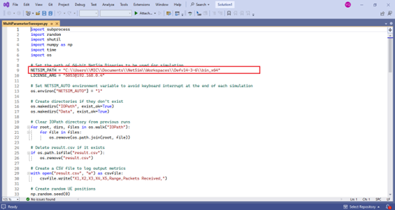
Figure-23: MultiParameterSweeper.py opened in the Visual Studio editor window

12. Run MultiParameterSweeper.py using command prompt.

Figure-24: Command prompt window in MultiParameterSweeper.py

13. The multi-parameter sweeper runs a total of 2000 simulations, varying X-coordinates between nodes and all transmission range values. It generates an output file named "result.csv" to store the collected data. (It took us approximately 2 hours to complete all 2000 simulations; we used a machine with a i5 processor and with 8 GB RAM).

14. To obtain the number of times the network is connected from the results, similar Excel procedures as with 2Nodes can be followed.

Python code for obtaining \(\mathbf{p}_{\mathbf{c}}\) from the analytical expression

We recall that the theoretical formula for probability of network connectivity for \(n\) nodes is

\[p_{c}(n,\ z,\ r) = \ \frac{U_{c}(n,\ z,\ r)}{U(n,\ z)} = \ \sum_{k = 0}^{n - 1}\binom{n - 1}{k}( - 1)^{k}\frac{(z - kr)^{n}}{z^{n}}u(z - kr)\]

where \(u(z)\) is the unit step function i.e., \(u(z) = 0\) when \(z \leq 0\) and \(u(z) = 1\) when \(z > 0\).

Python Code for obtaining probability of network connectivity.

import numpy as np
import math
from scipy.special import comb

def unit_func(z):
    return 1 if z > 0 else 0

def analytical_probability(n):
    analytical_prob = []

    for j, r_z in enumerate(np.arange(0.05, 1.05, 0.05), start=1):
        pro = 0
        for k in range(n):
            pro += comb(n-1, k) * ((-1) ** k) * ((1 - k * r_z) ** n) * unit_func(1 - k * r_z)

        analytical_prob.append(round(pro, 3))  # Rounding to 3 decimals

    print(analytical_prob)
    return analytical_prob

# Example usage
n = 10  # Replace with your desired value
analytical_probability(n)

Results

The values in the table below for the columns marked “Analysis” are calculated using the python code provided above, with n (the number of nodes) as an input to the python function.

Normalized transmission range \(\mathbf{(r/z)}\)	Network Connectivity Fraction (N=2)		Network Connectivity Fraction (N=5)		Network Connectivity Fraction (N=10)		Network Connectivity Fraction (N=20)
	Sim.	Analysis	Sim.	Analysis	Sim.	Analysis	Sim.	Analysis
0.05	0.09	0.097	0.00	0.001	0.00	0.000	0.00	0.000
0.10	0.16	0.190	0.00	0.010	0.00	0.002	0.03	0.019
0.15	0.23	0.277	0.06	0.043	0.06	0.045	0.39	0.393
0.20	0.34	0.360	0.15	0.115	0.21	0.243	0.77	0.787
0.25	0.42	0.437	0.32	0.234	0.53	0.528	0.91	0.939
0.30	0.47	0.510	0.43	0.389	0.72	0.750	0.99	0.984
0.35	0.56	0.577	0.6	0.550	0.9	0.879	1	0.996
0.40	0.63	0.640	0.77	0.691	0.94	0.946	1.00	0.999
0.45	0.68	0.697	0.82	0.799	0.97	0.977	1.00	0.999
0.50	0.73	0.750	0.92	0.875	1.00	0.991	1.00	1.00
0.55	0.78	0.797	0.95	0.926	1.00	0.997	1.00	1.00
0.60	0.85	0.840	0.95	0.959	1.00	0.999	1.00	1.00
0.65	0.87	0.877	0.98	0.979	1.00	1.00	1.00	1.00
0.70	0.88	0.910	1.00	0.990	1.00	1.00	1.00	1.00
0.75	0.94	0.937	1.00	0.996	1.00	1.00	1.00	1.00
0.80	0.95	0.960	1.00	0.999	1.00	1.00	1.00	1.00
0.85	0.99	0.977	1.00	1.00	1.00	1.00	1.00	1.00
0.90	1.00	0.990	1.00	1.00	1.00	1.00	1.00	1.00
0.95	1.00	0.997	1.00	1.00	1.00	1.00	1.00	1.00
1.00	1.00	1.000	1.00	1.00	1.00	1.00	1.00	1.00

Table-3: Results of NetSim simulation and analysis for N= 2, 5, 10 and 20 nodes. The network connectivity fraction is the ratio of number of times the network is connected to the total number of simulations runs.

Figure-25: Plot comparing simulation results against analytical model for probability of network connectivity for different transmission ranges.

Exercises

1. Configure NetSim simulations for node counts such as 3, 4, 6, 7, 8 etc. Then tabulate the output results containing Network connectivity for various Normalized Transmission Ranges using NetSim simulation, and from the closed form expression provided. Plot the results and compare simulation results vs. theory.

References

[1] A. Kumar, D. Manjunath and J. Kuri, Wireless Networking, Morgan Kaufmann, 2008.