Simulation GUI
In the Main menu select New Simulation \(\rightarrow\) Wireless Sensor Networks as shown in Figure 2-1.

Create Scenario
Fast Configuration

Fast Config window allows users to define device placement strategies and conveniently model large network scenarios especially in networks such as MANET, WSN and IoT. The parameters associated with the Fast Config Window are explained below:
(i) Grid Origin: The ‘Grid Origin’ refers to the intersection point of the system’s axes. NetSim supports any (X, Y) setting for the origin and not just (0, 0)
(ii) Grid Dimension: The width parameter represents the maximum along X from the origin and the height parameter represents the maximum along Y from the origin
(iii) Device placement area: The “Device Placement Area” allows users to specify the width and length of the area where devices are used when using the auto placement utility. This area must be less than or equal to the “Grid Area”.
Device Placement – Automatic Placement:
Uniform Placement: Devices will be placed uniformly with equal gap between the devices in area as specified inside length. This requires users to specify the number of devices as square number. For example, 1, 4, 9, 16 etc.
Random Placement: Devices will be placed randomly in the grid environment within the area as specified inside length.
File Based Placement: To place devices in user defined locations file-based placement option can be used. The file has the following general format:
<DEVICE NAME>,<DEVICE TYPE>,<X COORDINATE>,<Y COORDINATE>
Where, DEVICE_NAME is any name that will be assigned to the device. And DEVICE_TYPE is the unique Device Identifier specific to each type of device in NetSim.
The following table provides a list of all possible devices in MANET, WSN, UWAN and IOT Networks that support the Fast Configuration along with their respective device types:
| NETWORK | DEVICE TYPE |
|---|---|
| MANET | Wireless Node Omni Antenna \(|\) Wireless Node Sector Antenna \(|\) Wired Bridge Node \(|\) Wireless Bridge Node \(|\) Wired Node \(|\) Router \(|\) L2 Switch |
| WSN | Sensors \(|\) Sink node |
| UWAN | Under Water node |
| IOT | IoT Sensors \(|\) Gateway \(|\) Wired Node \(|\) IoT Router \(|\) Access Point |
NOTE: For more details about File Based Placement, refer 3.6.
Number of Devices: It is the total number of devices that are to be placed in the grid environment. It should be a square number in case of Uniform placement.
Manually Via Click and Drop: Selecting this option will load a grid environment with an ad hoc link where users can add devices manually by clicking and dropping the devices as required.
Wireless Sensor Networks
The devices that are involved in WSN are:
Wireless Sensor: In general, sensors monitor and record the physical conditions of the environment which is then sent to a central location (Sink node) where the data is collated and analyzed for further action. Sensors in NetSim are abstract in terms of what they sense, and NetSim focuses on the network communication aspects after sensing is performed.
WSN Sink (in WSN): Sink node is the principal controller in WSN. All sensors send their data to this sink node. In NetSim, users can drop only one sink node in a WSN.
Ad-hoc Link: Ad hoc link depicts a decentralized type of wireless network. The network is ad hoc because it does not rely on any pre-existing infrastructure, such as routers in wired networks or access points in managed wireless networks. In NetSim, Ad hoc links are used to connect the Sensors and the Sink node. Ad hoc links are used here for a visual representation of connection of all the devices in an Ad hoc basis.

NOTE: While designing a network, by default an ad hoc link will be present in the scenario. Click sensor nodes and sink nodes present in the ribbon/toolbar and drop them inside the grid. If the auto-connect option in the status bar is turned ON, these devices will be automatically connected to the ad hoc link. Refer section 3.2.3 of User Manual to know more about Auto Connection.
Internet of Things
The devices that are involved in IoT are:
IoT Sensor: In general, sensors monitor and record the physical conditions of the environment which is then sent to a central location (Lowpan Gateway) where the data is collated and analyzed for further action. Sensors in NetSim are abstract in terms of what they sense, and NetSim focuses on the network communication aspects after sensing is performed.
LoWPAN Gateway (in IoT): LoWPAN is an acronym of Low power Wireless Personal Area Networks. The LoWPAN IoT gateway functions as a border router in a LoWPAN network, connecting a wireless IPv6 network to the Internet. The wired portion of the network in IoT runs IPv4 whereas the wireless portion runs IPv6. The IPv6 routing protocols supported are AODV and RPL.
Ad-hoc Link: Ad hoc link depicts a decentralized type of wireless network. The network is ad hoc because it does not rely on any pre-existing infrastructure, such as routers in wired networks or access points in managed wireless networks. In NetSim IoT, Ad hoc links are used to connect the IoT Sensors and the LowPAN Gateway. Ad hoc links are used here for a visual representation of connection of all the devices in an Ad hoc basis.
Users can also add routers and nodes as shown below. Routers can be connected to the LoWPAN-Gateway and nodes/switches can be connected to routers using wired/wireless links.
Differences between IoT and WSN in NetSim
| WSN | IoT |
|---|---|
| WSN is a network of sensors and a sink node. | IOT has a gateway which can be used to connect to internetworks (having routers, switches, APs etc.). |
| WSN runs IPv4 and features a sink (not a gateway). | IOT runs IPv6 in the sensor network (802.15.4 MAC/PHY) and IPv4 on the inter-network portion. |
| Routing protocols in NetSim WSN include, DSR, AODV, OLSR, and ZRP. | Routing protocols in NetSim IoT include, AODV and RPL. |
NOTE: Refer MANET Technology library for working of AODV, DSR, OLSR and ZRP.
Device Attributes
GENERAL PROPERTIES
Right click on any sensor and open properties as new window. The general properties of the sensor are:
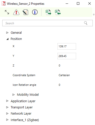
Device name – It is the name of sensor which is editable and will reflect in the GUI before and after simulation.
X and Y – These are the coordinates of a sensor.
Z co-ordinate – By default this will be zero and is reserved for future use.
Interface count is 1 since sensors share the wireless Multipoint-to-Multipoint medium.
Mobility Models: Mobility models can be used to model movement of sensors. The mobility models provided in NetSim are:
Random Walk Mobility model: It is a simple mobility model based on random directions and speeds.
Random Waypoint Mobility Model: It includes pause time between changes in direction and/or speed.
Group mobility: It is a model which describes the behavior of sensors as they move together i.e., the sensors having common group id will move together.
Pedestrian Mobility Model: This model is applicable to each node (local parameter), and the configuration parameters are:
Pedestrian Max Speed (m/s) (Range: 0.0 to 10.0. Default: 3.0)
Pedestrian Min Speed (m/s) (Range: 0.0 to 10.0. Default: 1.0)
Pedestrian stop probability (Range: 0 to 1)
Pedestrian stop duration (s) (Range: 1 to 10000)
In this model it is assumed that the pedestrian stops at traffic lights. The stop probability represents the probability of encountering a traffic light. This is checked for every calculation interval. Once stopped, the pedestrian waits for a duration equal to stop duration for the light to turn green. A new direction is chosen randomly after every stop with \(\theta\) (angle between new direction and current direction) taking values of 0, 90, 180, 270. These \(\theta\) values represent the pedestrian continuing in the same direction, taking a left, taking a U turn and taking a right respectively.
A new speed is chosen randomly after every stop. Min speed \(\leq\) Speed \(\leq\) Max speed.
The maximum number of stops and starts is 10.
File Based mobility: In File Based Mobility, users can write their own custom mobility models and define the movement of the mobile users. The name of the trace file generated should be kept as mobility.csv and it should be in the NetSim Mobility File format.
APPLICATION PROPERTIES – Transport Protocol, by default set to UDP. To run with TCP, users have to select TCP protocol from the drop down.
NETWORK LAYER – NetSim WSN, supports the following MANET routing protocols.
DSR (Dynamic source routing): Note that in wireless sensor networks, by default Link Layer Ack is enabled. If Network Layer ack is enabled users must set DSR ACK in addition to Zigbee ACK in MAC layer.
AODV (Ad-hoc on-demand distance vector routing):
ZRP (Zone routing protocol): For interior routing mechanism NetSim uses OLSR protocol.
OLSR (Optimized link State Routing): Except zone radius all the parameters are similar to ZRP.

AODV – AODV (Ad Hoc on Demand Distance Vector) is an on-demand routing protocol for wireless networks that uses traditional routing tables to store routing information. AODV uses timers at each node and expires the routing table entry after the route is not used for a certain time.
Some of the features implemented in NetSim are:
RREQ, RREP and RERR messages.
Hello message.
Interface with other MAC/PHY protocols such as 802.15.4, TDMA / DTDMA.
Hello interval – It describes the interval in which it will discover its neighbor routes.
Refresh interval – It is the duration after which each active node periodically refreshes routes to itself.
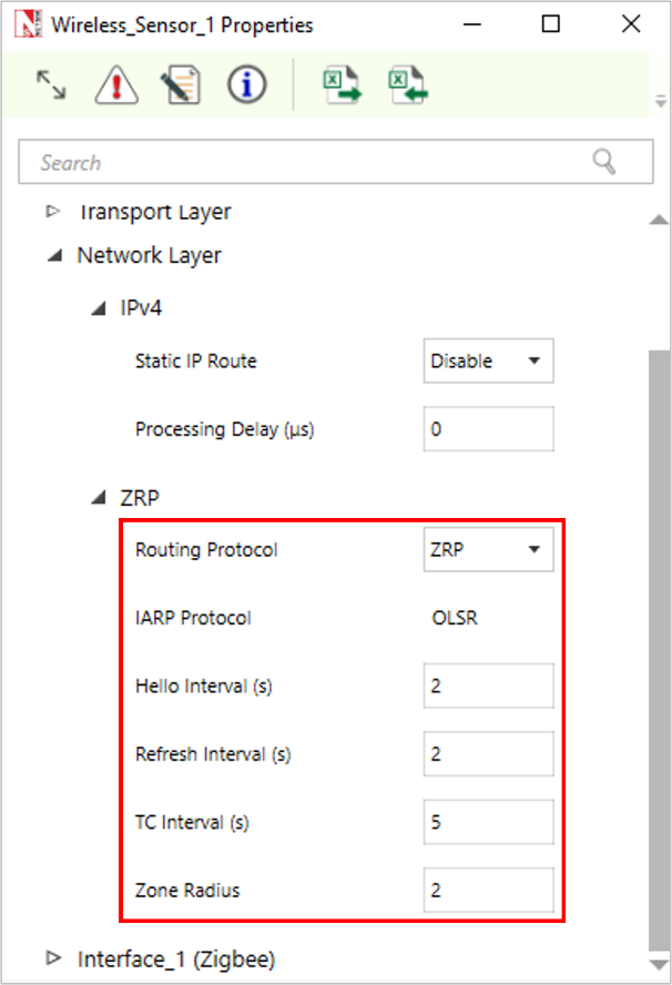
Topology Control messages – These are the link state signaling done by OLSR. These messages are sent at TC interval every time.
Zone radius – After dividing the network range of the divided network will be based on zone radius. A node’s routing zone is defined as a collection of nodes whose minimum distance in hops from the node in question is no greater than a parameter referred to as the zone radius.
DATALINK LAYER
802.15.4 (Zigbee Protocol) runs in MAC layer. In the sink node or pan coordinator properties users can configure the Beacon frames and the Superframe structure.

Superframe Order – It describes the length of the active portion of the Superframe, which includes the beacon frame. Range is from 0–15.
Beacon Order – Describes the interval at which coordinate shall transmit its beacon frames. Range is from 1–15.
GTS Mode (Guaranteed Time Slot) – If it is enabled it allows a device to operate on the channel within a portion of the super frame that is dedicated (on the PAN) exclusively to the device.
Battery life Extension – This subfield is 1 bit in length and shall be set to one if frames transmitted to the beaconing device.
Superframe Duration – It is divided into 16 equally sized time slots, during which data transmission is allowed. The value of super-frame duration by default is 15.36ms.
Max CSMA Backoff – It is the maximum number of attempts the CSMA-CA algorithm will make before declaring a channel access failure. Having range 0–5.
Minimum CAP length – It is the minimum number of symbols forming the Contention access period. This ensures that MAC commands can still be transferred to devices when GTSs (Guaranteed time slots) are being used.
Max and Min Backoff Exponent – Values of CSMA-CA algorithms have a range of 3–5.
Max Frame Retries – It is the total number of retries after failed attempts.
Unit Backoff Period – It is the number of symbols forming the basic time period used by the CSMA-CA algorithms.
PHYSICAL LAYER
The frequency band used in NetSim WSN simulations is 2.4 GHz, and the bandwidth is 5 MHz. NetSim simulates a single channel ZigBee network and does not support multiple channels.
Data rate – It is the number of bits that are processed per unit of time. The data rate is fixed at 250 kbps per the 802.15.4 standard.
Chip Rate – A chip is a pulse of direct sequence spread spectrum code, so the chip rate is the rate at which the information signal bits are transmitted as pseudo random sequence of chips.
Modulation technique – O-QPSK (Offset quadrature phase shift keying), sometimes called staggered quadrature phase shift keying, is a variant of phase-shift keying modulation using 4 different values of the phase to transmit.
MinLIFSPeriod – It is the minimum long inter-frame spacing period. It is the time difference between short frame and long frame in unacknowledged case and the time difference between short frame and acknowledged case in acknowledgment transmission.
SIFS (Short inter-frame Symbol) – It is generally the time for which receiver waits before sending the CTS (Clear To Send) & acknowledgement packet to sender, and sender waits after receiving CTS and before sending data to receiver. Its main purpose is to avoid any type of collision. Min SIFS period is the minimum number of symbols forming a SIFS period.
Phy SHR duration – It is the duration of the synchronization header (SHR) in symbol for the current PHY.
Phy Symbol per Octet – It is the number of symbols per octet for the current PHY.
Turn Around Time – Transmitter to receiver or receiver to transmitter turnaround time is defined as the shortest time possible at the air interface from the trailing edge of the last chip (of the first symbol) of a transmitted PLCP protocol data unit to the leading edge of the first chip (of the first symbol) of the next received PPDU.
CCA (Clear Channel Assessment) – It is a carrier sensing mechanism in Wireless Networks. The different types of CCA modes available are:
Carrier Sense Only: It shall report a busy medium only upon the detection of a signal compliant with this standard with the same modulation and spreading characteristics of the PHY that is currently in use by the device. This signal may be above or below the ED threshold.
Energy Detection: It shall report a busy medium upon detecting signal strength above the ED threshold.
Carrier Sense with Energy Detection: It shall report a busy medium using a logical combination of detection of a signal with the modulation and spreading characteristics of this standard and Energy above the ED threshold, where the logical operator may be AND or OR.
Receiver sensitivity – It is the minimum magnitude of input signal required to produce a specified output signal having a specified signal-to-noise ratio, or other specified criteria. It is up to the user to determine the desired receiver sensitivity.
Receiver ED threshold – It is intended for use by a network layer as part of channel selection algorithms. It is an estimate of the received signal power within the bandwidth of the channel. No attempt is made to identify or decode signal on the channel. If the received signal power is greater than the ED threshold value, then the channel selection algorithms will return false.
Transmitter Power – It is the signal intensity of the transmitter. The higher the power radiated by the transmitter’s antenna, the greater the reliability of the communication system. The connection medium is wireless.
POWER MODEL
Power source – It can be battery or main line. This model in NetSim is used for energy calculations. In case of battery, the following parameters will be considered:
Recharging current – It is the current flow during recharging. Range is from 0–1000mA.
Energy harvesting – It is the process by which energy is derived from external source, captured, and stored. NetSim supports an abstract Energy Harvesting model. A specified amount of energy, calculated from recharging current and voltage specified, is added to the remaining energy of the node periodically to replenish the battery. It can be turned on or off.
Initial Energy – It is the battery energy. Range is from 0.001–3250mAh.
Transmitting current – It is the current for transmitting power. Range is 0–1000mA. Transmit power and transmit current are independent in NetSim. Since the focus of NetSim is packet simulation, the power modeling is abstract. It is left to the user to change the transmit current accordingly, when increasing or decreasing the transmit power, if the user’s goal is to study power consumption.
Idle mode – It is the current flow during the idle mode. Range is between 0–1000mA.
Voltage – It is a measure of the energy carried by the charge. Range is from 0–10V.
Receiving current – It is the current required to receive the data, ranging from 0–1000mA.
Sleep mode current – It is the current flowing in sleep mode of battery. Range is from 0–1000mA.
NOTE: The resultant energy metrics and their definitions are provided in the NetSim User Manual in the Outputs section.
The following table shows the properties of sensor in NetSim.
| Property | Default Setting |
|---|---|
| Network layer | |
| Routing protocol | DSR |
| ACK_Type | LINK_LAYER_ACK |
| Data link layer | |
| ACK request | Enable |
| Max Csma BO | 4 |
| Max Backoff Exponent | 5 |
| Min Backoff Exponent | 3 |
| Max frame retries | 3 |
| Local properties (and Default settings) | |
| Physical layer | |
| phySHRduration(symbols) | 3 |
| Physymbolperoctet | 5.3 |
| CCA mode | CARRIER SENSE ONLY |
| Receiver sensitivity(dbm) | \(-85\) |
| ED threshold (dbm) | \(-95\) |
| Transmitter power(mW) | 1 |
| Power | |
| Power source | Battery |
| Energy harvesting | ON |
| Recharging current (mA) | 0.4 |
| Initial energy (mAH) | 300 |
| Transmitting current (mA) | 17 |
| Idle mode current (mA) | 3.3 |
| Voltage (v) | 3.6 |
| Receiving current (mA) | 9.6 |
| Sleep mode current (mA) | 0.237 |
Set Node, Link and Application Properties
Users need to connect the sensors and LoWPAN gateway using links.
Interconnection among other devices is same as in Internetworks.
LoWPAN gateway can be connected with router using links.
Click on the appropriate node or link to open its properties in the property panel on the right. Then modify the parameters according to the requirements.
Routing protocol in Application Layer of routers and all user editable properties in Datalink layer and Physical Layer of Access Point and Wireless Node are Global/Local.
In Sensor node, Routing protocol in Network Layer and all user editable properties in Datalink layer, Physical Layer and Power are Global/Local.
NOTE:
Global – Changing properties in one node will automatically reflect in any other nodes in that network.
Local – Changing properties in one node will not reflect in any other nodes in that network.
The following are the main properties of sensor node in PHY and Datalink layers as shown in Figure 2-9/Figure 2-10/Figure 2-11.


Set the values according to requirement and proceed.
Click on the Set Traffic tab present on the top ribbon and select an application.

Set the application properties as per the requirements and proceed.

Detailed information on Application properties is available in section 6 of NetSim User Manual.
Setting Static Routes
In Device Properties \(\triangleright\) Network layer \(\triangleright\) Static IP Route, users can set static routes. When static routes are set the dynamic routing protocol entries are overwritten by the static routing entries. Static route configuration is explained in the Internetworks technology library document, Section Configuring Static Routing in NetSim.
Static route option is available for all sensors in WSN.

The Static routes option is not available in the wireless portion of the IoT network as IoT devices work with IPv6 network addressing. The devices present in the wired portion of the network may have IPv4 addressing. Hence static routes can be configured in the wired section (till the gateway) of an IoT network.
Configure Reports
Enable Packet Trace, Event Trace (Optional)
Check Packet Trace / Event Trace option from the Configure Reports tab. To get detailed help, please refer to sections 8.4 and 8.5 in User Manual.

Enable protocol specific plots
Click on “Plots” icon in the top ribbon from “Configure Reports” tab, which will then open a right plot panel, containing a list of available plots for the network as chosen by the user.
Check boxes can be enabled to generate the respective plots. To get detailed help, please refer to section 8.2 in User Manual.

Enable protocol specific logs
Users can enable protocol specific log files such as the Radio Measurement log, Energy log etc., by clicking on the Configure Reports tab and selecting Plot icon option present in the toolbar.
Check boxes can be enabled to generate the respective logs. To get detailed help, please refer to section 8.3 in the User Manual.

GUI Configuration Parameters
| Parameter | Scope | Range | Description |
|---|---|---|---|
| Ack Request | Local | Enable or Disable | The Ack Request setting allows a device to
control whether it wants a confirmation (acknowledgment) that its
message has been received. Enable Ack Request: When this is turned on, every time the device sends a message, it includes a request for acknowledgment (Ack) in the message’s control information. The recipient must send back a confirmation message (an acknowledgment) to let the sender know the message was successfully received. Disable Ack Request: When this is turned off, the device sends messages without asking for confirmation, so the recipient does not send an acknowledgment back. |
| Mac Address | Fixed | The MAC address is a unique value associated with a network adapter. This is also known as hardware address or physical address. This is a 12-digit hexadecimal number (48 bits in length). | |
| MAC CSMA Backoff | Local | 0–5 | The maximum number of backoffs the CSMA-CA algorithm will attempt before declaring a channel access failure. |
| Maximum Backoff Exponent | Local | 3–8 | The maximum value of the backoff exponent (BE) in the CSMA-CA algorithm. |
| Minimum Backoff Exponent | Local | 3–8 | The minimum value of the backoff exponent (BE) in the CSMA-CA algorithm |
| Max Frame retries | Local | 0–7 | The maximum number of retries allowed after a transmission failure. |
| Unit Backoff Period | Fixed | 20 | The number of symbols forming the basic time period used by the CSMA-CA algorithm |
| Sinknode-Interface(Wireless) – Datalink Layer | |||
| Beacon Mode | Local | Enable / Disable | Beacon Mode is a setting that affects how
a network stays in sync and manages reliable communication: Enable Beacon Mode: When Beacon Mode is turned on, the network sends regular signals (called “beacons”) to keep all devices synchronized. This improves reliability because all devices know when they can send and receive messages, making communication more organized. Disable Beacon Mode (Beaconless): When Beacon Mode is turned off, devices communicate using a simpler method called CSMA-CA (Carrier Sense Multiple Access with Collision Avoidance). This approach is lighter and requires less coordination, but it may be less reliable since devices try to avoid message collisions. |
| Superframe Order | Local | 0–15 | Superframe Order describes the length of the active portion of the superframe, which includes the beacon frame. |
| Beacon Order | Local | 1–15 | Beacon Order, describes the interval at which the coordinator shall transmit its beacon frames. |
| GTS Mode | Local | Enable/ Disable | GTS Mode (Guaranteed Time Slot Mode) is a
setting that decides if a device gets its own reserved time to
communicate on the network: Enable GTS Mode: When GTS Mode is enabled, a specific time slot within the network’s schedule (superframe) is reserved just for the device. This dedicated time slot means the device can use the channel without interference from others, ensuring reliable and uninterrupted communication. Disable GTS Mode: When GTS Mode is off, the device shares the channel with other devices without a dedicated time slot, which may cause it to wait or experience interruptions. |
| Battery Life Extension | Local | TRUE/False | The Battery Life Extension (BLE) setting
is a single on/off switch (1 bit) that helps save battery by controlling
when devices send data after a beacon signal. BLE set to 1 (On): When BLE is turned on, devices must send data to the main device (beaconing device) within a short, specific time after the beacon signal. This short time window, known as the “backoff period,” helps the device finish communication quickly, saving battery by reducing how long it stays active. BLE set to 0 (Off): When BLE is off, there is no strict time limit on when the device must start sending data after the beacon. This uses more battery because the device may stay active longer, but it allows more flexibility in timing. |
| Superframe Duration (ms) | Local | 15.36 | Superframe Duration is divided into 16 equally sized time slots, during which data transmission is allowed. The value of super-frame duration by default is 15.36ms. |
| Interface Wireless – Physical Layer | |||
| Data Rate (Kbps) | Fixed | Data rate or bit rate is the number of bits that are conveyed or processed per unit of time. | |
| Chip Rate | Fixed | The chip rate of a code is the number of pulses per second (chips per second) at which the code is transmitted (or received). The chip rate is larger than the symbol rate, meaning that one symbol is represented by multiple chips. | |
| Symbol Rate | Fixed | In digital communications, symbol rate (also known as baud or modulation rate) is the number of symbol changes (waveform changes or signaling events) made to the transmission medium per second using a digitally modulated signal or a line code. | |
| Modulation Technique | Fixed | O-QPSK (Offset quadrature phase shift keying) sometimes called as staggered quadrature phase shift keying is a variant of phase-shift keying modulation using 4 different values of the phase to transmit. | |
| Min LIFS Period | Fixed | The minimum number of symbols forming a LIFS (Long Inter Frame Spacing) period. | |
| Min SIFS Period | Fixed | The minimum number of symbols forming a SIFS (Short Inter Frame Spacing) period. | |
| Phy SHR duration | Local | 3,7,10,40 | Phy SHR duration is the duration of the synchronization header (SHR) in symbol for the current PHY |
| Phy Symbol per Octet | Fixed | Phy Symbol per Octet is number of symbols per octet for the current PHY | |
| Turn Around Time | Fixed | Turnaround Time is the minimum wait time needed for a device to switch from sending to receiving data (or vice versa) in a wireless network. | |
| CCA Mode | Local | CCA (Clear Channel Assessment) is a
carrier sensing mechanism in Wireless Networks. The different types of
CCA modes available are: Carrier Sense Only: It shall report a busy medium only upon the detection of a signal compliant with this standard with the same modulation and spreading characteristics of the PHY that is currently in use by the device. This signal may be above or below the ED threshold Energy Detection: It shall report a busy medium upon detecting signal strength above the ED threshold. Carrier Sense with Energy Detection: It shall report a busy medium using a logical combination of detection of a signal with the modulation and spreading characteristics of this standard and Energy above the ED threshold, where the logical operator may be AND or OR. |
|
| Receiver sensitivity | Local | \(-999\) to 0 | Receiver sensitivity is the minimum magnitude of input signal required to produce a specified output signal having a specified signal-to-noise ratio, or other specified criteria. It is up to the user to determine the desired receiver sensitivity. |
| ED threshold(dBm) | Local | \(-999\) to 0 | The receiver ED threshold is intended for use by a network layer as part of a channel selection algorithm. It is an estimate of the received signal power within the bandwidth of the channel. No attempt is made to identify or decode signals on the channel. If the receive signal power is greater than the ED threshold value then the channel selection algorithm will return false. |
| Transmitter Power (mW) | Local | 1 to 100 | It is the signal intensity of the transmitter. The higher the power radiated by the transmitter’s antenna the greater the reliability of the communications system. |
| Antenna Gain (dBi) | Local | \(-1000\) to 1000 | A relative measure of an antenna’s ability to direct or concentrate radio frequency energy in a particular direction or pattern. The measurement is typically measured in dBi (Decibels relative to an isotropic radiator). |
| Antenna Height (m) | Local | 0 to 100 | Antenna height is used in the pathloss calculation in the following models: Cost231 Hata Urban, Cost231 Hata SubUrban, Hata Urban, Hata SubUrban and Two Ray. This parameter has no effect when using any of the other pathloss models. |
| Power Source | Local | Main Line or Battery | Sensor communicate with each other using battery power. By default, the power model is set to Main Line, which represents a general-purpose alternating current (AC) electric power supply. The power model is user-configurable, with adjustable properties. |
| Energy Harvesting | Local | On or Off | Energy harvesting is the process of
deriving energy from external sources (e.g., solar power, thermal
energy, wind energy, and kinetic energy), capturing it, and storing it
for use in small, wireless autonomous devices, such as those in wearable
electronics and wireless sensor networks. NetSim supports an abstract energy harvesting model in which a specified amount of energy (calculated from the recharging current and specified voltage) is periodically added to the remaining energy of the node to replenish the battery. This feature can be turned on or off. |
| Initial Energy | Local | 0.001–3250 mAh | A node has an initial value which is the level of energy the node has at the beginning of the simulation. |
| Transmitting Current | Local | 0–10000 mA | In the Transmitting mode (Tx mode), the node consumes energy to transfer packets or data. The amount of energy consumed in this mode depends on the number of packets sent by the node, greater the number of packets, the more energy is consumed. |
| Idle Mode Current | Local | 0–1000 mA | In idle mode, a node doesn’t transmit or receive data but still listens to the wireless medium for potential packets and new nodes. This consumes less energy than sending or receiving, as no active communication occurs. |
| Voltage | Local | 0–10 V | Voltage is a measure of the energy carried by the charge. |
| Receiving Current | Local | 0–1000 mA | In the Receiving mode (Rx mode), the nodes are actively listening to the incoming data, it consumes the energy as it receives the data from the sender. |
| Recharging Current | Local | 0–1000 mA | Recharging Current refers to the flow of electric charge supplied to a battery during the recharging process |
| SleepMode Current | Local | 0–1000mA | Current flow during sleep mode. |
| Network Layer | |||
| Routing Protocol | Global | RPL, AODV, DSR, ZRP, OLSR | |
| RPL Routing Protocol | |||
| Instance ID | Global | 1 to 20 | It is a unique identifier within a network. DODAGs with the same RPL Instance ID share the same Objective Function. |
| Node Type | Fixed | Router | A DAG root is a node within the DAG that has no outgoing edges. Because the graph is acyclic, all DAGs must have at least one DAG root and all paths terminate at a DAG root. LowPAN gateway is the root device. Any sensors can be configured as a Router or Leaf. If a node is configured to act as a router, it starts advertising the graph information with the new information to its neighboring peers. If the node is a “leaf node”, it simply joins the graph and does not send any DIO message. |
| DAO Delay (s) | Global | 0–20 | A node should delay sending the DAO message to aggregate DAO information from other nodes for which it is a DAO parent. Receiving a DAO message starts the Delay DAO timer. DAO messages received while the Delay DAO timer is active do not reset the timer. When the Delay DAO timer expires, the node sends a DAO. |
| DIS Initial Delay (ms) | Global | 1–1000 | The time for which the node waits before sending DIS message. |
| DIS Interval (ms) | Global | 1–1000 | DIS Interval is the time interval between two DIS messages |
| DSR Routing Protocol | |||
| ACK Type | Global | LINK_LAYER_ACK or NETWORK_LAYER_ACK | The user can enable either Link Layer ACK
(Layer 2 ACK) or Network Layer ACK (Layer 3 ACK). Link Layer ACK uses
MAC layer acknowledgment for route maintenance, while Network Layer ACK
uses DSR acknowledgment for route maintenance. For more details, refer to sections 3.2.1 and 3.2.2 of the MANET Technology Library. |
| ZRP and OLSR Routing Protocol | |||
| Hello Interval | Global | 1–100 s | Hello interval parameter is used for neighbor discovery process. This parameter determines how frequently Hello messages are sent out and also how frequently a neighbor table will be updated. |
| Refresh Interval | Global | 1–100 s | Refresh interval is the duration after which each active node periodically refreshes routes to itself. |
| IARP | Fixed | IARP is used by a node to communicate with the interior nodes of its zone and is limited by the zone radius. | |
| TC Interval | Global | 1–100 s | Topology Control messages are the link state signaling done by OLSR. These messages are sent at TC interval every time. |
| Zone radius | Global | 2–225 m | Zone radius parameter is present for ZRP
Protocol. ZRP divides the entire network into zones. The radius of these zones is defined by Zone radius. |
Run Simulation
Click on the Run Simulation icon on the top toolbar.

Set the Simulation Time and click on Run.