Featured Examples
Sample configuration files for all networks are available in the Examples Menu in NetSim Home Screen. These files provide examples on how NetSim can be used – the parameters that can be changed and the typical effect it has on performance.
IOT
Energy Model
Open NetSim, Select Examples \(\triangleright\)IOT-WSN \(\triangleright\)Internet of Things \(\triangleright\)Energy Model then click on the tile in the middle panel to load the example as shown in Figure 4-1.

The following network diagram illustrates what the NetSim UI displays when you open the example configuration file.

Settings done in sample network:
Grid is set to 1000 \(\times\) 500 from grid setting property panel on the right. This needs to be done before any device is placed on the grid.
Click on LOWPAN Gateway and expand the right property panel, enable the Beacon Mode and change the Superframe Order to 12 and the Beacon Order to 12 under the Interface 1 (Zigbee) layer.

Click on sensor, go to physical layer in Interface (Zigbee) layer and change the power source to Battery.
Click on link and open property panel on the right and set the channel characteristics \(\rightarrow\) No pathloss in Ad hoc link Properties.
Configure a sensor application between Sensor 2 and Wired node 4 from the Set Traffic tab in ribbon on the top.
Enable the sleep energy vs time plot by clicking on configure reports tab \(\triangleright\) Plots and run the simulate for 50 sec.
In Simulation metrics window, click on Additional metrics in the left panel and check the Battery model metrics, users should get zero value for Sleep energy (mJ) consumed.
Go back to Simulation window change following properties in LOWPAN Gateway for another sample.
Set Superframe Order (SO) and Beacon Order (BO) as 10 and 12 respectively (\(0 \leq SO \leq BO \leq 14\)).
Re-run the Simulate for 50 sec.
Results:
In the simulation results window click on additional metrics on the left and scroll down for the Battery model metrics for both the cases.
In Superframe order 12 and Beacon order 12 Sample, users can observe sleep energy consumed value will be zero in Battery model metrics since sensor is in active state all the time, i.e., if SO=12 and BO=12, there won’t be any inactive portion of the Superframe.

Similarly, open the Sleep energy vs time plot from simulation results window, compare the sleep energy consumed by sensor over the simulation time for both cases when SO =12 and BO =12 and SO =10 and BO =12.

In Superframe order 10 and Beacon order 12 Sample, sleep energy consumed will be non-zero since sensor goes to sleep mode during the inactive portion of the Superframe.


Working of RPL Protocol in IoT
Open NetSim, Select Examples \(\triangleright\)IOT-WSN \(\triangleright\)Internet of Things \(\triangleright\)Working of RPL Protocol in IoT then click on the tile in the middle panel to load the example as shown in Figure 4-8.
The following network diagram illustrates what the NetSim UI displays when you open the example configuration file.

Settings done in sample network:
Set grid length as 120 \(\times\) 60m from grid setting property panel on the right. This needs to be done before any device is placed on the grid.
Click on LOWPAN Gateway or sensor. In the right property panel, change the routing protocol to RPL under network layer as shown in Figure 4-10.

Click on link, expand the right property panel change Channel characteristics \(\rightarrow\) Path Loss only, Path Loss Model \(\rightarrow\) Log Distance and path loss exponent \(\rightarrow\) 3.5.
Configure sensor applications as shown in the below table by clicking on set traffic tab from the ribbon on the top.
| Application ID | Application Type | Source Id | Destination Id |
|---|---|---|---|
| 1 | SENSOR APP | 1 | 8 |
| 2 | SENSOR APP | 3 | 8 |
| 3 | SENSOR APP | 5 | 8 |
Procedure to get detailed RPL log file:
Go to help option in the title bar.
Click on Open Source code.
Go to the RPL Project in the Solution Explorer. Open RPL.h file and change
// #define DEBUG_RPLto#define DEBUG_RPLas shown in Figure 4-11.

Right click on the RPL project in the solution explorer and click on rebuild.
After the RPL project is rebuilt successfully, go back to the network scenario.
Enable the Application throughput vs time and Link throughput vs time plots under plots in configure reports tab and run simulation for 100 sec and go to Result window \(\rightarrow\) Logs, open rpl log file.


Note:
Detailed information of the RPL log file is available for the standard version of NetSim. For academic users, the rank value can be observed by enabling Wireshark and also python script is available to know the parent and sibling information. Please find the below link to download and run the python utility: https://support.tetcos.com/support/solutions/articles/14000134056-how-to-visualize-the-rpl-dodag-in-netsim-iot-simulations-
The observations of rpl log file which is generated in NetSim is given in the below Table 4-2.
| Node | Rank | Updated Rank | Parent list | Updated Parent Node ID | Sibling Node ID | Received DIO From Node ID |
|---|---|---|---|---|---|---|
| Node 1 | 30 | 27 | Node 2, Node 4 | Node 2 | Node 3 | Node 2, Node 3, Node 4 |
| Node 2 | 15 | 15 | Node 6 | Node 6 | Node 4 | Node 4, Node 6 |
| Node 3 | 28 | 28 | Node 2, Node 4, Node 5 | Node 4 | Node 1 | Node 1, Node 2, Node 4, Node 5 |
| Node 4 | 15 | 15 | Node 6 | Node 6 | Node 2 | Node 2, Node 6 |
| Node 5 | 27 | 27 | Node 4 | Node 4 | – | Node 4 |
The above table can be summarized as follows:
DIO message is sent by the root node, i.e. LowPAN Gateway, with Rank 1 to Sensor 2 and Sensor 4 as shown in Figure 4-14.

On receiving the DIO message, Node 4 will recognize the DODAG Id of Root Node and identifies it as Parent node. Rank of Node 4 will get updated to 15. Also, Node 2 is recognized as sibling of Node 4.
Now, node 4 will broadcast DIO message to other nodes as shown in Figure 4-15.

Node 1 receives DIO message from Node 4 and it identifies the DODAG Id of Node 4. Hence, Node 1 recognizes Node 4 as the Parent Node. Rank of Node 1 will get updated to 30. As Node 3 is within the range of Node 1, Node 3 is identified as a sibling of Node 1.
Node 1 will then broadcast DIO messages as shown in Figure 4-16.

Node 2 receives the DIO message from Node 6 and identifies it as Parent node. The Rank of Node 2 gets updated to 15. Node 2 now broadcasts the DIO message to other nodes as shown in Figure 4-17.

Node 3 receives DIO message from Node 4 and the rank of Node 3 gets updated to 28. Node 4 is identified as the parent node of Node 3.
Node 3 then broadcasts DIO message to other nodes as shown in Figure 4-18.

Node 5 receives DIO message from Node 3, hence, it identifies Node 4 as the parent node. The rank of Node 5 gets updated to 27.
Node 5 then broadcasts DIO message as shown in Figure 4-19.

Further, Node 1 receives DIO message from Node 2 and the parent list of Node 1 gets updated to Node 4 and Node 2. Also, the rank of Node 1 gets updated to 27.
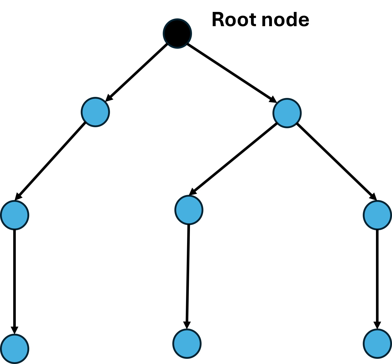
According to the link quality, DODAG is formed.
Node 2 and Node 4 are siblings and their parent is Node 6 (Root Node). Rank is 15.
Node 1 and Node 3 are siblings.
Node 1 establishes its parent as Node 2. Rank is 27.
Node 3 establishes its parent as Node 4. Rank is 28.
Node 5 doesn’t have any siblings and establishes its parent as Node 4. Its rank is 27.

Modes of Operation in IoT RPL
The DODAG nodes process the DAO messages according to the RPL Mode of Operations (MOP), which are presented below. Independent of the MOP used, DAO messages may require reception confirmation, which should be done using DAO-ACK messages.
Although it is designed for the Multipoint-to-Point (MP2P) traffic pattern, RPL also admits the data forwarding using Point-to-Multipoint (P2MP) and Point-to-Point (P2P). In MP2P, the nodes send data messages to the root, creating an upward flow as shown in Figure 4-21. In P2MP, sometimes termed as multicast, the root sends data messages to the other nodes, producing a downward flow depicted in Figure 4-23.
In P2P, a node sends messages to the other node (non-root) of DODAG; thus, both upward and downward forwarding may be required as illustrated in Figure 4-22. RPL defines four MOPs that should be used considering the traffic pattern required by the application and the computational capacity of the nodes. In the first, MOP 0 (Point to multipoint), RPL does not maintain downward routes; thus, consequently, only MP2P traffic is enabled. In storing without multicast MOP (MOP 2 (Point to point)), downward routes are also supported, but are different from MOP 1; the nodes maintain, individually, a routing table constructed using DAO messages to provide downward traffic. Hence, downward forwarding occurs without the use of the root node, as illustrated in Figure 4-24. Storing with multicast has a functioning similar to MOP 2 (Point to point) plus the possibility of multicast data sending. This type of transmission permits the non-root node to send messages to a group of nodes formed using multicast DAOs.


Open NetSim, Select Examples \(\triangleright\)IOT-WSN \(\triangleright\)Internet of Things \(\triangleright\)Mode of Operations IoT RPL then click on the tile in the middle panel to load the example as shown in Figure 4-25.

The following network diagram illustrates what the NetSim UI displays when you open the example configuration file.

Multipoint to Point
Settings done in sample network:
Set grid length as 200 \(\times\) 100m from grid setting property panel on the right. This needs to be done before any device is placed on the grid.
Routing protocol has been set as RPL for LOWPAN Gateway and Sensor. Click on device, expand the right-side property panel and go to Network Layer set Routing Protocol as shown in Figure 4-27.
Click on the link, expand the right-side property panel, and set the channel characteristics to ‘Path Loss Only’. Then, set the path loss model to ‘Log Distance’ and the path loss exponent to 4.2.
Configure sensor applications as shown in the below table by clicking on set traffic tab from the ribbon on the top.
| Application ID | Application Type | Source Id | Destination Id |
|---|---|---|---|
| 1 | SENSOR APP | 1 | 11 |
| 2 | SENSOR APP | 3 | 11 |
| 3 | SENSOR APP | 8 | 11 |
In NetSim GUI Packet Traces and Plots are Enabled. Run simulation 100s and observe that all the sensors are sending data to the root node in packet trace.
Result
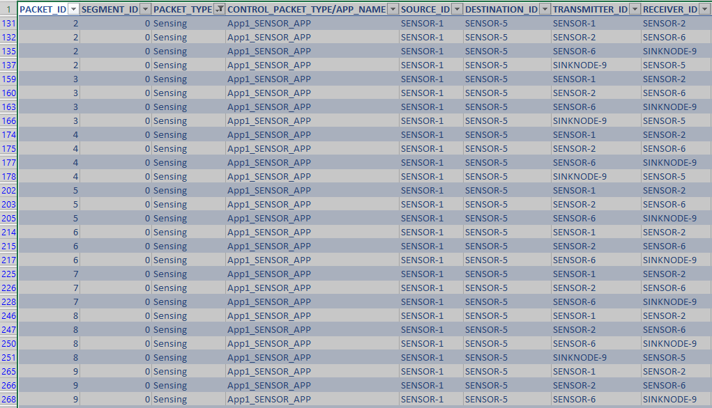
Packet trace: The nodes send data messages to the root, creating an upward flow which can be observed in the packet trace. Once the simulation is completed, to view the packet trace file, click on “Packet Trace” under Traces option present in the left-hand-side of the Simulation Results Dashboard and filter the PACKET TYPE to Sensing. You can observe the flow of Sensor Application packets as shown in Figure 4-28.

Point to Multipoint
Settings done in sample network:
Set all the properties the same as Multipoint to Point scenario.
Configure sensor applications as shown in the below table by clicking on set traffic tab from the ribbon on the top.
| Application ID | Application Type | Source Id | Destination Id |
|---|---|---|---|
| 1 | SENSOR APP | 11 | 1 |
| 2 | SENSOR APP | 11 | 3 |
| 3 | SENSOR APP | 11 | 8 |
Run simulation 100s and observe that all the sensors are sending data to the root node in packet trace.
Result
Packet trace: Root sends data messages to the other nodes, producing a downward flow which can be observed in the packet trace. Once the simulation is completed, to view the packet trace file, click on “Packet Trace” under Traces option present in the left-hand-side of the Simulation Results Dashboard and filter the PACKET TYPE to Sensing, you can observe the flow of Sensor Application packets as shown below:

Point to Point
Settings done in sample network:
Set all the properties the same as Multipoint to Point scenario.
Configure sensor applications as shown in the below table by clicking on set traffic tab from the ribbon on the top.
| Application ID | Application Type | Source Id | Destination Id |
|---|---|---|---|
| 1 | SENSOR APP | 1 | 5 |
Run simulation 100s and observe that all the sensors are sending data to the root node in packet trace.
Result
Packet trace: Root sends data messages to the other nodes, producing a downward flow which can be observed in the packet trace. Once the simulation is completed, to view the packet trace file, click on “Packet Trace” under Traces option present in the left-hand-side of the Simulation Results Dashboard and filter the PACKET TYPE to Sensing, you can observe the flow of Sensor Application packets as shown below:
Storing Mode
Settings done in sample network:
Set all the properties the same as Multipoint to Point scenario.
Configure sensor applications as shown in the below table by clicking on set traffic tab from the ribbon on the top.
| Application ID | Application Type | Source Id | Destination Id |
|---|---|---|---|
| 1 | SENSOR APP | 3 | 8 |
Run simulation 100s and observe that all the sensors are sending data to root node in packet trace.
Result
In storing without multicast MOP (MOP 2 (Point to point)), downward routes are also supported, but are different from MOP 1 (Point to multipoint); the nodes maintain, individually, a routing table constructed using DAO messages to provide downward traffic. Hence, downward forwarding occurs without the use of the root node. The results can be analyzed from the packet trace.
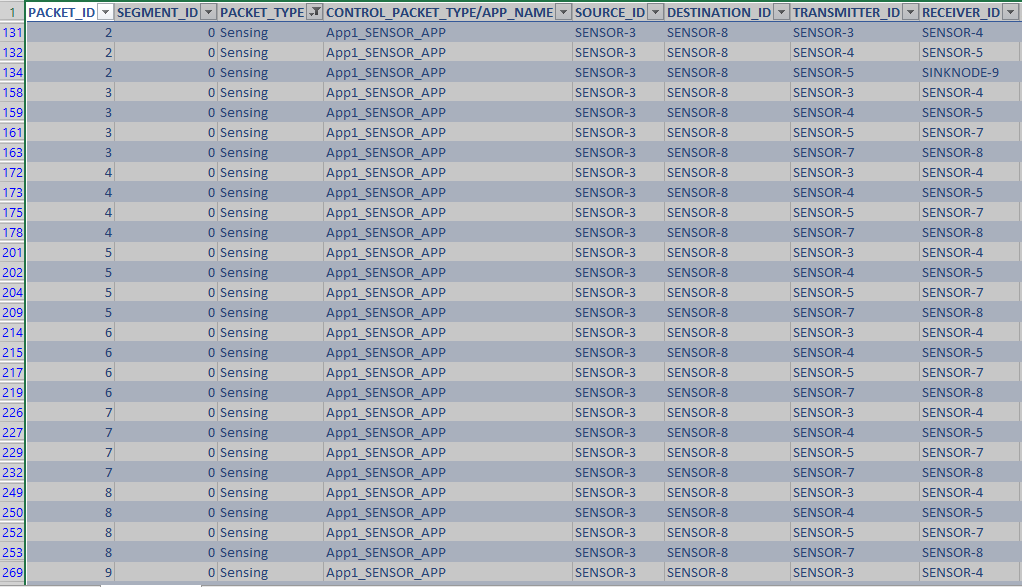
Packet trace: Once the simulation is completed, to view the packet trace file, click on “Packet Trace” under Traces option present in the left-hand-side of the Simulation Results Dashboard and filter the PACKET TYPE to Sensing, you can observe the flow of Sensor Application packets as shown below.
DDoS attack in an IoT Network
Introduction
A DoS (Denial of Service) attack in IoT (Internet of Things) involves overwhelming a device or network with traffic to disrupt its normal operation and deny service to legitimate users. This can be achieved by flooding the network with a large volume of traffic or sending packets with malformed headers to exploit vulnerabilities in the target system. The impact of a DoS attack on an IoT device or network can be significant, as many IoT devices have limited processing power and memory resources. As a result, they may not be able to handle the large volume of traffic generated by the attack, leading to service disruptions or even device failures. When multiple attackers coordinate a DoS attack, it is known as a DDoS (Distributed Denial of Service) attack.
Botnet Attack
A botnet attack in IoT (Internet of Things) is a type of cyber-attack where a network of compromised IoT devices, such as smart home appliances, security cameras, and routers, is used to carry out malicious activities. In a botnet attack, a hacker gains control of a large number of IoT devices, often through exploiting vulnerabilities or weak security measures, and uses them to launch coordinated attacks.
Once a hacker has control of a botnet, they can carry out a variety of malicious activities, including:
DDoS attacks: A distributed denial-of-service (DDoS) attack floods a website or network with traffic, making it unavailable to legitimate users.
Data theft: A hacker can use a botnet to steal sensitive data, such as financial information or personal data, from devices on the network.
Spamming: A botnet can be used to send large volumes of spam emails or messages.
Crypto mining: A hacker can use a botnet to mine cryptocurrency using the processing power of compromised devices.
Bit-and-piece Attack
A “bit and piece” DDoS attack in an IoT network is a type of Distributed Denial of Service (DDoS) attack that targets Internet of Things (IoT) devices by sending small amounts of traffic to a large number of devices. This type of attack is also known as a low-rate DDoS attack.
In a bit-and-piece attack, the attacker sends a small amount of traffic to multiple IoT devices, such as smart home appliances, security cameras, or routers. The traffic may include a range of packet types, such as TCP, UDP, and ICMP, and the packets may be sent intermittently over a long period of time. Because the traffic is distributed across many devices, each individual device receives a small amount of traffic that is difficult to distinguish from legitimate traffic. However, when combined, the traffic overwhelms the network and causes a denial of service for legitimate users trying to access the network.
Network Setup for Botnet Attack
Case 1: Without Malicious Node (No attacker)
In NetSim, click on Examples \(\triangleright\) IOT-WSN \(\triangleright\) DDoS attack in an IOT Network

Drop 9 Sensors, 1 LOWPAN gateway, 1 router, and 1 wired node(Server) as shown in the figure.
Click on the sensor, expand the property panel on right and set the routing protocol to RPL.
Click on the link and expand the link property panel on the right. Set the channel characteristics to Path Loss only, Path Loss Model to Log Distance, and path loss exponent to 4.5.
Configure sensor traffic from all sensors to server by clicking on set traffic tab in ribbon on top, such that the packets are transmitted to the gateway via sensor 9. The traffic rate is low; it is 20 packets per second. Set Transport Protocol to UDP, Packet size = 50 Bytes and IAT (\(\mu\)s) = 50000
Run the simulation for 100 seconds and measure the throughput obtained by sensors 1 through 8.
Case 2: With a Malicious Node (DoS attack node)

Configure traffic from all sensors 1 through 8 such that the packets are transmitted to the gateway via sensor 9. The traffic rate is low; it is 20 packets per second. Set Transport Protocol to UDP, Packet size = 50 Bytes and IAT (\(\mu\)s) = 50000
Add a malicious node. Configure traffic such that packets are transferred via sensor 9. This has a “high” generation rate to flood the network; it is 1000 packets per second. Set Packet size = 50 Bytes and IAT (\(\mu\)s) = 1000
Run the simulation for 100 seconds and measure the throughput obtained by sensors 1 through 8.
Results and Observation
| Application | Case 1 – Normal Operation Throughput (Mbps) | Case 2 – DoS Attack Throughput (Mbps) |
|---|---|---|
| Sensor 1 | 0.003789 | 0.000712 |
| Sensor 2 | 0.001201 | 0.000192 |
| Sensor 3 | 0.004383 | 0.00076 |
| Sensor 4 | 0.007476 | 0.001221 |
| Sensor 5 | 0.005849 | 0.003633 |
| Sensor 6 | 0.004195 | 0.003338 |
| Sensor 7 | 0.001424 | 0.001544 |
| Sensor 8 | 0.006226 | 0.004386 |
| Malicious Node | N/A | 0.014886 |
| Sum Throughput (Mbps) Sensor 1 through 8 | 0.034543 (34.54 Kbps) | 0.015786 (15.78 Kbps) |
From the table, we observe that the introduction of the malicious node led to a more than 50% drop in throughput, from 34.54 Kbps to 15.78 Kbps.
Network Setup for Bit-and-Piece Attack
In NetSim, click on Examples \(\triangleright\) IOT-WSN \(\triangleright\) DDoS attack in an IOT Network
Case 1: Without Malicious Node (No attacker)

Drop 10 sensors, 1 LOWPAN Gateway, 1 Router and 1 Wired node (server) as shown in the figure.
Click on the sensor, expand the property panel on right and set the routing protocol to RPL.
Click on the link and expand the link property panel on the right. Set the channel characteristics to Path Loss only, Path Loss Model to Log Distance, and path loss exponent to 4.5.
Configure 9 applications. Each application is from a sensor (1, 2, \(\ldots\), 9) to the server, such that packets of size 50 Bytes are sent at a rate of 20 packets/sec. Set Transport Protocol to UDP, Packet size = 50 Bytes and IAT (\(\mu\)s) = 50000
The network topology and routing are such that traffic from all sensors flows through relay (sensor 10), and then to the gateway and onwards to the server.
Run the simulation for 100 seconds and measure the throughput obtained by sensors 1 through 9.
We then simulate 3 attack cases.


Case 2: Add 1 malicious node (wired). Configure custom traffic from malicious node to all sensors (1, 2, \(\ldots\), 9). Packets of size 10 Bytes (representing a small amount of attack data) are sent at a rate of 20 packets/sec exponentially. Set Transport Protocol to UDP, Packet Size = 10 Bytes and exponential distribution for IAT (\(\mu\)s) = 50000.
Case 3: Add 2 malicious nodes (wired). Configure custom traffic from 2 malicious nodes to all sensors (1, 2, \(\ldots\), 9). Packets of size 10 Bytes (representing a small amount of attack data) are sent at a rate of 20 packets/sec exponentially. Set Transport Protocol to UDP, Packet Size = 10 Bytes and exponential distribution for IAT (\(\mu\)s) = 50000.
Case 4: Add 3 malicious nodes (wired). Configure custom traffic from 3 malicious nodes to all sensors (1, 2, \(\ldots\), 9). Packets of size 10 Bytes (representing a small amount of attack data) are sent at a rate of 20 packets/sec exponentially. Set Transport Protocol to UDP, Packet Size = 10 Bytes and exponential distribution for IAT (\(\mu\)s) = 50000.
Run the simulation for 100 seconds and measure the throughput obtained by sensors 1 through 9 in each case.
Results and Observation
| Application | Case 1: Normal Operation Throughput (Mbps) | Case 2: 1 attacker node Throughput (Mbps) | Case 3: 2 attacker nodes Throughput (Mbps) | Case 4: 3 attacker nodes Throughput (Mbps) |
|---|---|---|---|---|
| Sensor 1 | 0.003577 | 0.002401 | 0.001968 | 0.001752 |
| Sensor 2 | 0.000853 | 0.000672 | 0.000596 | 0.00048 |
| Sensor 3 | 0.002185 | 0.001577 | 0.001445 | 0.001233 |
| Sensor 4 | 0.007332 | 0.004942 | 0.003966 | 0.003546 |
| Sensor 5 | 0.004501 | 0.003417 | 0.002724 | 0.002428 |
| Sensor 6 | 0.004527 | 0.00317 | 0.002582 | 0.002242 |
| Sensor 7 | 0.001184 | 0.000976 | 0.000788 | 0.000672 |
| Sensor 8 | 0.006346 | 0.004406 | 0.003609 | 0.002953 |
| Sensor 9 | 0.002189 | 0.001625 | 0.001329 | 0.001089 |
| Sum Throughput (Mbps) of Legitimate Traffic | 0.032694 (32.6 Kbps) | 0.023186 (23.1 Kbps) | 0.019007 (19.1 Kbps) | 0.016395 (16.3 Kbps) |
We observe:
25% drop in throughput of legitimate traffic with 1 bit-and-piece DDoS attack node.
50% drop in throughput of legitimate traffic with 3 bit-and-piece DDoS attack nodes.
WSN
Beacon Time Analysis
Open NetSim, Select Examples \(\triangleright\)IOT-WSN \(\triangleright\)Wireless Sensor Networks \(\triangleright\)Beacon Time Analysis, then click on the tile in the middle panel to load the example as shown in Figure 4-38.

The following network diagram illustrates what the NetSim UI displays when you open the example configuration file.

Settings done in sample config file
The following grid properties are already set, as Manually Via Click and Drop.
In the SinkNode, the Super frame mode and Beacon mode are set to 10 and 12, respectively. To configure it, click on the SinkNode. On the right side, expand the property panel, go to the data link layer of the Interface (Zigbee) layer, and set the Superframe Order (SO) to 10 and the Beacon Order (BO) to 12.

In the position layer of wireless sensors and the sink, the mobility model is set to Random Waypoint.
In Adhoc link properties change the channel characteristics as Path Loss only, Path Loss Model to Log Distance and path loss exponent as 2.
Create sensor traffic between Wireless Sensor 1 and WSN Sink 3 from the Set Traffic tab in the top ribbon. Click on the created application, set the transport layer protocol to UDP, and leave the other properties as default.
Enable Packet trace from the configure report tab in the ribbon on the top.

Run the simulation for 200 seconds.
Theoretical Beacon Time Calculation
Beacon Interval (BI) = Superframe duration (SD) + Inactive Period (IP). The Superframe duration (SD) is also known as the Active period.
\(BI = aBaseSuperframe\ duration\times {2}^{BO} = 15.36ms \times {2}^{12} = 62914.56ms \approx 62s.\)
\(SD = aBaseSuperframe\ duration\times {2}^{SO} = 15.36ms \times {2}^{10} = 15728.64ms.\)
\(aBaseSuperframe\ duration\) is a constant defined by the standard and is equal to \(15.36 ms\)
To find Inactive period, \(IP = BI - SD = 62914.56ms - 15728.64ms = 47185.92ms.\)
Superframe duration is divided into 16 slots (1st slot is allocated for beacon frame).
Each slot time \(=\frac{15728.64ms}{16} = 983.04ms\)
NetSim Results:
Open packet trace and filter CONTROL PACKET TYPE to Zigbee BEACON FRAME, users should get four Zigbee beacon frames at 0, 62.9, 125.8, 188.7 secs (approx.) for each Sensor Node, because the time interval between two beacon frames is 62 seconds. Since we have 2 nodes, the user can get 4 beacon frames for each node.

4 beacons were transmitted, so \(beacon\ time = 983.04ms\times 4 = 3932.16\ millisec\) (since 1 beacon = 1 time slot). Check the beacon time in IEEE 802.15.4 metrics window.
CAP Time Analysis
Open NetSim, Select Examples \(\triangleright\)IOT-WSN \(\triangleright\)Wireless Sensor Networks \(\triangleright\)CAP Time Analysis, then click on the tile in the middle panel to load the example as shown in Figure 4-43.

The following network diagram illustrates what the NetSim UI displays when you open the example configuration file.

Settings done in example config file
The following grid properties are already set, as Manually Via Click and Drop.
In the SinkNode, the Super frame mode and Beacon mode are set to 10 and 12, respectively. To configure it, click on the SinkNode. On the right side, expand the property panel, go to the data link layer of the Interface (Zigbee) layer, and set the Superframe Order (SO) to 10 and the Beacon Order (BO) to 12.

In the position layer of wireless sensors and the sink, the mobility model is set to Random Waypoint.
In Adhoc Link Properties change Channel characteristics \(\triangleright\) Path Loss only, Path Loss Model \(\triangleright\) Log Distance and path loss exponent \(\triangleright\) 2.
Create sensor traffic between Wireless Sensor 1 and WSN Sink 3 from the Set Traffic tab in the top ribbon. Click on the created application, set the transport layer protocol to UDP, and leave the other properties as default.
Enable Packet trace from the configure report in the ribbon on the top.
Run the Simulation for 100 sec.
Theoretical CAP Time Calculation
To find CAP time, BI is 62914.56ms \(\triangleright\) So in 100s, two beacon frames should be transmitted at 0 & 62s.
Check no. of beacon frames transmitted in 802.15.4 metrics.
Here CFP = 0 because there is only 1 sensor.
\(CAP\ Time = SD - beacon\ time = (15728.64ms) - (983.04ms) = 14745.6ms.\)
Open packet trace and filter Control Packet Type to Zigbee Beacon Frame, users should get two ZigBee beacon frames at 0, 62.9secs, because the time interval between two beacon frames is 62 seconds. Since we have 2 nodes, the user can get 2 beacon frames for each node.
Since two Beacon frames are transmitted,
\[CAP\ time = 2\times 14745.6ms = 29491200\ \mu s.\]
NetSim Results:
In the NetSim simulation results window, click on Additional Metrics and scroll down to the IEEE 802.15.4 Metrics table. Compare the theoretical CAP time with the CAP time in the IEEE 802.15.4 Metrics table.
CAP time = 29491200.0000 Microsec.

Static Routing in WSN
Open NetSim, Select Examples \(\triangleright\)IOT-WSN \(\triangleright\)Wireless Sensor Networks \(\triangleright\)WSN Static Route then click on the tile in the middle panel to load the example as shown in Figure 4-47.

The following network diagram illustrates what the NetSim UI displays when you open the example configuration file.

Case 01: Without Static Route
Settings done in the network
The following grid properties are already set, as Manually via Click and Drop.
The sensor application is created between Sensor 1 and 6 from the Set Traffic tab in the top ribbon.
Packet trace is enabled from the configure reports tab.
Simulation time is set to 100 sec.
Results: Open the packet trace and observe the data flow. Sensor 1 sends packets directly to Sinknode 6.

Case 02: With Static Route
Settings done in the network.
For the above sample (without static route), we have configured the static routes for sensors. The following steps explain how to configure static routes.
Configuring Static Routes
Click on the wireless sensor 1. In the right property panel, go to the network layer under IPv4 and enable Static IP Route.
Then, click on via GUI in Configure Static IP Route and set the Network Destination, Gateway, Subnet Mask, Metrics, and Interface ID as shown in the screenshot below. Click add and then OK.

Similarly, configure static routes for other sensors as follows:
| Device | Network Destination | Gateway | Subnet Mask | Metrics | Interface ID |
|---|---|---|---|---|---|
| Wireless Sensor 1 | 192.168.0.7 | 192.168.0.3 | 255.255.255.0 | 1 | 1 |
| Wireless Sensor 2 | 192.168.0.7 | 192.168.0.4 | 255.255.255.0 | 1 | 1 |
| Wireless Sensor 3 | 192.168.0.7 | 192.168.0.5 | 255.255.255.0 | 1 | 1 |
| Wireless Sensor 4 | 192.168.0.7 | 192.168.0.6 | 255.255.255.0 | 1 | 1 |
| Wireless Sensor 5 | 192.168.0.7 | 192.168.0.7 | 255.255.255.0 | 1 | 1 |
After setting the properties click on run simulation for 100 sec.
Results
Open the packet trace and observe the packet flow. The data will be transmitted according to the statically configured routes.
SENSOR 1 \(\rightarrow\) SENSOR 2 \(\rightarrow\) SENSOR 3 \(\rightarrow\) SENSOR 4 \(\rightarrow\) SENSOR 5 \(\rightarrow\) SINK NODE

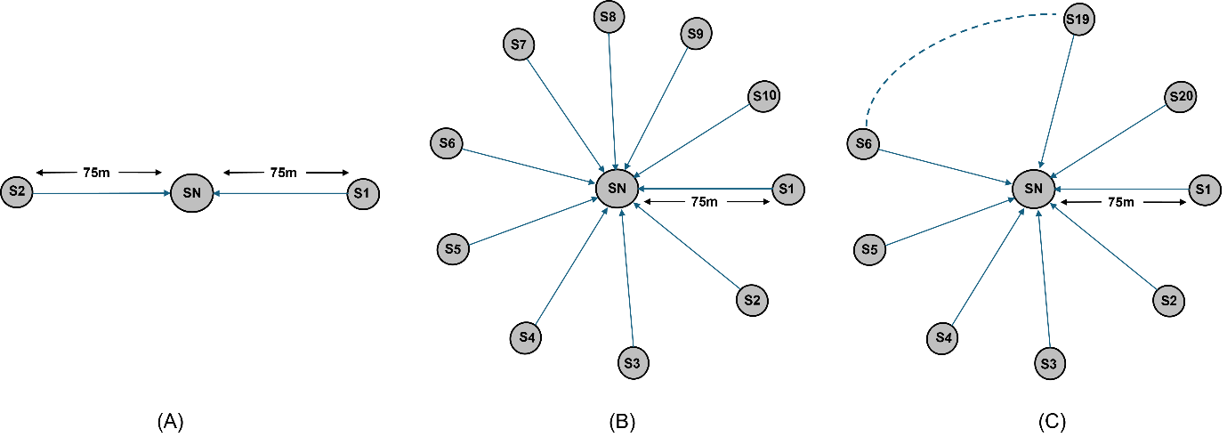
Analysing throughput, latency and energy consumption as we scale the number of sensors
We examine a scenario in which sensors are arranged in a circular configuration around a central sink, with all sensors positioned within the carrier sense range of each other. As the number of sensors increases, we analyse throughput, latency, and energy consumption in ZigBee’s (802.15.4) beaconless and beacon enabled modes across different packet sizes.
Network Layout
Network Scenario
Open NetSim, Select Examples \(\triangleright\) IOT-WSN \(\triangleright\) Wireless Sensor Networks \(\triangleright\) Analyzing throughput, latency and energy consumption as we scale the number of sensors \(\triangleright\) Analyzing Throughput, Latency, and Energy Consumption in Beacon-Disabled Mode and then click on the tile in the middle panel to load the example as shown in Figure 4-53.

The following network diagram illustrates what the NetSim UI displays when you open the example configuration file.

Case 1:
Create a scenario with 2 Sensor nodes and 1 Sink node.
Distance between the sensors and sink nodes should be 75m.
Click on Sink node and expand the property panel on right side and disable the beacon mode in datalink layer of Interface (Zigbee) properties.
| Device Properties | |
|---|---|
| Network layer properties | |
| Routing protocol | DSR |
| Interface (Wireless) properties | |
| Physical layer properties | |
| ED Threshold (dBm) | \(-87\) |
| Power | Battery |
Similarly repeat this step for all other sensors.
Configure the Static Route from Sensors to Sink Node as shown below.
Static routes were configured in each source node such that the data gets transmitted directly from source to destination without any dynamic route formation by the routing protocols.
Static routes (whereby \({N}_{i}\) always transmits to \({N}_{(i+1)}\)) are set to ensure single hop transmission. Thereby each node transmits data to the next-hop node according to the topology.
To set the static routes, go to Wireless Sensor properties \(\triangleright\) Network Layer \(\triangleright\) Enable Static Route IP and click on Configure static route via GUI and update as below.

The Static route IPs were configured in Wireless Sensor 1, Wireless Sensor 2, Wireless Sensor 3 etc. and Wireless Sensor 20 as shown below:
| Device | Network Destination | Gateway | Subnet Mask | Metrics | Interface ID |
|---|---|---|---|---|---|
| Wireless Sensor 1 | 192.168.0.1 | 192.168.0.1 | 255.255.255.255 | 1 | 1 |
| Wireless Sensor 2 | 192.168.0.1 | 192.168.0.1 | 255.255.255.255 | 1 | 1 |
| Wireless Sensor 3 | 192.168.0.1 | 192.168.0.1 | 255.255.255.255 | 1 | 1 |
| Wireless Sensor 4 | 192.168.0.1 | 192.168.0.1 | 255.255.255.255 | 1 | 1 |
| Wireless Sensor \(i\) | 192.168.0.1 | 192.168.0.1 | 255.255.255.255 | 1 | 1 |
| Wireless Sensor 20 | 192.168.0.1 | 192.168.0.1 | 255.255.255.255 | 1 | 1 |
Create a CUSTOM application from Sensor to Sink Node by clicking on set traffic tab from the ribbon on the top. Click on created application and expand application property on right panel, set packet size to 50 bytes and Inter arrival time to 100000 \(\mu\)s.
Run the Simulation for 1000 seconds.
Similarly increase the number of nodes to 4, 6, 8, 10, 12, 14, 16, 18, 20 and record the results.
Results
Case 1: Beacon Mode Disabled (Low Latency)
Results for throughput and latency can be observed from the application metrics window of simulation results window and to observe transmit energy, receive energy and idle energy, click on additional metrics in the left and scroll down to the battery model metrics.

| Number of sensor nodes | Avg. Transmit Energy (mJ) | Avg. Receive Energy (mJ) | Avg. Idle Energy (mJ) | Average Throughput (Mbps) | Aggregate Throughput (Mbps) | Average Latency (Delay) (\(\mu\)s) |
|---|---|---|---|---|---|---|
| 2 | 1860.16 | 0.00 | 11517.82 | 0.0035 | 0.0070 | 6768 |
| 4 | 1829.45 | 0.00 | 11523.87 | 0.0032 | 0.0128 | 10566 |
| 6 | 1726.93 | 0.00 | 11543.78 | 0.0028 | 0.0167 | 12927 |
| 8 | 1596.88 | 0.00 | 11569.16 | 0.0024 | 0.0190 | 14317 |
| 10 | 1476.38 | 0.00 | 11592.55 | 0.0020 | 0.0204 | 15255 |
| 12 | 1377.65 | 0.00 | 11611.73 | 0.0017 | 0.0208 | 15999 |
| 14 | 1298.89 | 0.00 | 11626.97 | 0.0015 | 0.0209 | 16651 |
| 16 | 1228.78 | 0.00 | 11640.55 | 0.0013 | 0.0210 | 17190 |
| 18 | 1174.44 | 0.00 | 11651.14 | 0.0012 | 0.0208 | 17683 |
| 20 | 1127.08 | 0.00 | 11660.36 | 0.0010 | 0.0203 | 18167 |


Discussion
The aggregate throughput increases initially but then decreases by increasing the number of nodes. The initial increase is because for small number-of-nodes the contention is less and increasing the node count increases the channel utilization.
With beacon mode disabled, all nodes remain active throughout the simulation, constantly ready to receive or transmit data. The transmitting energy per node decreases as more nodes are added to the network, which is due to the distribution of transmissions among more sensors. However, this operational mode results in a high average idle energy as nodes consume power even when they are not actively transmitting data.
This transmission mode is suitable for applications that prioritize low latency over energy efficiency.
Network Scenario
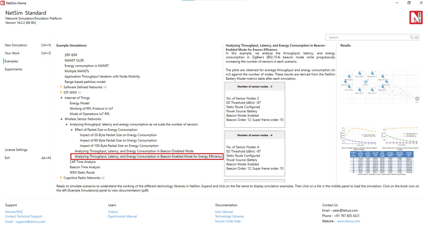
Open NetSim, Select Examples \(\triangleright\) IOT-WSN \(\triangleright\)Wireless Sensor Networks \(\triangleright\) Analyzing throughput, latency and energy consumption as we scale the number of sensors \(\triangleright\) Analyzing Throughput, Latency, and Energy Consumption in Beacon-Enabled Mode for Energy Efficiency then click on the tile in the middle panel to load the example as shown in Figure 4-60.
Case 2:
Consider the same scenario as Case 1
Go to Sink Node \(\triangleright\) Interface ZIGBEE \(\triangleright\) Datalink Layer, Set the Beacon Mode to Enable and Set the Beacon Order to 12 and Super frame Order 10.
Run the Simulation for 1000 seconds.
Results
Case 2: Beacon Mode Enabled (Energy efficiency)
| No. of nodes | Avg. Tx Energy (mJ) | Avg. Rx Energy (mJ) | Avg. Idle Energy (mJ) | Avg. Sleep Energy (mJ) | Avg. Throughput (Mbps) | Agg. Throughput (Mbps) | Avg. Latency (\(\mu\)s) |
|---|---|---|---|---|---|---|---|
| 2 | 1703.73 | 0.2831 | 2658.87 | 638.39 | 0.0032 | 0.0065 | 20442177 |
| 4 | 1479.89 | 0.2831 | 2702.32 | 638.39 | 0.0025 | 0.0098 | 20668437 |
| 6 | 1282.07 | 0.2831 | 2740.72 | 638.39 | 0.0019 | 0.0114 | 20627134 |
| 8 | 1137.54 | 0.2831 | 2768.78 | 638.39 | 0.0015 | 0.0118 | 20497185 |
| 10 | 1028.29 | 0.2831 | 2789.99 | 638.39 | 0.0012 | 0.0116 | 20454173 |
| 12 | 949.96 | 0.2831 | 2805.19 | 638.39 | 0.0009 | 0.0113 | 20261225 |
| 14 | 883.15 | 0.2831 | 2818.16 | 638.39 | 0.0008 | 0.0107 | 20173343 |
| 16 | 832.50 | 0.2831 | 2827.99 | 638.39 | 0.0006 | 0.0102 | 19829588 |
| 18 | 792.54 | 0.2831 | 2835.75 | 638.39 | 0.0005 | 0.0097 | 19779115 |
| 20 | 756.68 | 0.2831 | 2842.71 | 638.39 | 0.0005 | 0.0092 | 19432628 |


Discussion
Case 2 introduces beacon-enabled mode in the network, significantly altering energy consumption patterns and network performance. When beacon mode is enabled, nodes in the network operate with defined periods for active and sleep states. Nodes wake up at specific beacon intervals to transmit and receive data, and then go back to sleep. This operation significantly reduces the average idle energy consumption because nodes are not constantly powered on waiting to receive or transmit data. Instead, they spend a substantial portion of time in the low-power sleep state, which is reflected in the sleep energy metrics in the results.
However, this also introduces a substantial increase in average latency, as nodes must wait for their turn to transmit during the beacon intervals, leading to delays in packet forwarding. This is reflected in the latency values, which are orders of magnitude higher than in Case 1. Throughput slightly decreases compared to Case 1, which is due to the time spent in low-power states, reducing the effective transmission time.
This transmission mode is suitable for applications that prioritize energy efficiency over latency.
Network scenario
Open NetSim, Select Examples \(\triangleright\) IOT-WSN \(\triangleright\) Wireless Sensor Networks \(\triangleright\) Analyzing throughput, latency and energy consumption as we scale the number of sensors \(\triangleright\) Effect of Packet Size vs Energy Consumption, then click on the tile in the middle panel to load the example as shown in Figure 4-64.

Case 3: Effect of Packet Size vs Energy Consumption
Consider the same scenario as Case-2
Create a CUSTOM Application with Source ID as Sensor and Destination ID as Sink Node, with the Packet Size 20 Bytes and Inter Arrival Time 100000 \(\mu\)s.
Run the Simulation for 1000 seconds.
Record the results from results dashboard.
Similarly vary the packet size in application to 60B and 100B respectively.
Rerun the simulation for 1000 seconds. Record the results from the results dashboard.
Results
| No. of nodes | Pkt Size (B) | Avg. Tx Energy (mJ) | Avg. Rx Energy (mJ) | Avg. Idle Energy (mJ) | Avg. Sleep Energy (mJ) | Avg. Throughput (Mbps) | Agg. Throughput (Mbps) | Avg. Latency (\(\mu\)s) |
|---|---|---|---|---|---|---|---|---|
| 20 | 1200.53 | 0.28 | 2756.56 | 638.4 | 0.0014 | 0.0028 | 20319671 | |
| 4 | 20 | 1142.49 | 0.28 | 2767.83 | 638.4 | 0.0012 | 0.0047 | 21071912 |
| 6 | 20 | 1081.05 | 0.28 | 2779.75 | 638.4 | 0.001 | 0.0061 | 21440249 |
| 8 | 20 | 1023.47 | 0.28 | 2790.93 | 638.4 | 0.0009 | 0.0071 | 21903767 |
| 10 | 20 | 969.01 | 0.28 | 2801.5 | 638.4 | 0.0008 | 0.0078 | 22150841 |
| 12 | 20 | 919.89 | 0.28 | 2811.04 | 638.4 | 0.0007 | 0.0083 | 22737334 |
| 14 | 20 | 879.28 | 0.28 | 2818.92 | 638.4 | 0.0006 | 0.0084 | 22943219 |
| 16 | 20 | 839.94 | 0.28 | 2826.55 | 638.4 | 0.0005 | 0.0084 | 23845867 |
| 18 | 20 | 790.46 | 0.28 | 2836.16 | 638.4 | 0.0005 | 0.0082 | 33464665 |
| 20 | 20 | 746.35 | 0.28 | 2844.72 | 638.4 | 0.0004 | 0.0079 | 44959110 |
| 2 | 60 | 1898.03 | 0.28 | 2621.16 | 638.4 | 0.004 | 0.0081 | 20736084 |
| 4 | 60 | 1731.53 | 0.28 | 2653.48 | 638.4 | 0.0034 | 0.0135 | 21670506 |
| 6 | 60 | 1569.88 | 0.28 | 2684.86 | 638.4 | 0.0028 | 0.017 | 22822081 |
| 8 | 60 | 1424.32 | 0.28 | 2713.12 | 638.4 | 0.0024 | 0.0191 | 23630100 |
| 10 | 60 | 1223.77 | 0.28 | 2752.05 | 638.4 | 0.0019 | 0.0191 | 53919154 |
| 12 | 60 | 1074.47 | 0.28 | 2781.03 | 638.4 | 0.0016 | 0.0188 | 79323930 |
| 14 | 60 | 967.4 | 0.28 | 2801.81 | 638.4 | 0.0013 | 0.0185 | 95181466 |
| 16 | 60 | 885.83 | 0.28 | 2817.65 | 638.4 | 0.0011 | 0.0181 | 107682323 |
| 18 | 60 | 821.14 | 0.28 | 2830.21 | 638.4 | 0.001 | 0.0175 | 115764304 |
| 20 | 60 | 770.42 | 0.28 | 2840.05 | 638.4 | 0.0009 | 0.017 | 123905731 |
| 2 | 100 | 2556.55 | 0.28 | 2493.33 | 638.4 | 0.0067 | 0.0134 | 21258705 |
| 4 | 100 | 2231.26 | 0.28 | 2556.48 | 638.4 | 0.0053 | 0.0211 | 22658685 |
| 6 | 100 | 1919.71 | 0.28 | 2616.95 | 638.4 | 0.0042 | 0.0252 | 27512241 |
| 8 | 100 | 1545.9 | 0.28 | 2689.52 | 638.4 | 0.0031 | 0.025 | 73068592 |
| 10 | 100 | 1310.88 | 0.28 | 2735.14 | 638.4 | 0.0025 | 0.0246 | 100074374 |
| 12 | 100 | 1151.74 | 0.28 | 2766.03 | 638.4 | 0.002 | 0.0241 | 118197099 |
| 14 | 100 | 1035.23 | 0.28 | 2788.65 | 638.4 | 0.0017 | 0.0234 | 129367238 |
| 16 | 100 | 944.31 | 0.28 | 2806.3 | 638.4 | 0.0014 | 0.0229 | 138470037 |
| 18 | 100 | 876.48 | 0.28 | 2819.46 | 638.4 | 0.0012 | 0.0221 | 145188141 |
| 20 | 100 | 819.23 | 0.28 | 2830.58 | 638.4 | 0.0011 | 0.0214 | 150341336 |


Discussion
Table 4-14 presents detailed metrics for energy consumption, throughput, and latency across various numbers of nodes and packet sizes (20B, 60B, and 100B).
Throughput Observations:
Average Throughput: This metric decreases with the increase in the number of nodes for all packet sizes. As more nodes are added, the data transmission per node reduces, due to increased contention and collisions on the network.
Aggregate Throughput: In contrast to average throughput, aggregate throughput increases initially as the number of nodes increases but then starts to decrease as further nodes are added. The initial increase is because for small number-of-nodes the contention is less and increasing the node count increases the channel utilization. However, beyond a threshold with more nodes, the likelihood of collisions increases due to more frequent attempts to access the channel simultaneously.
Energy Consumption Observations:
Transmit Energy: Average transmit energy decreases as the number of nodes increases. This is due to the distribution of transmissions among more nodes.
Receive and Sleep energy: Receive energy and sleep energy remain relatively consistent across different numbers of nodes and packet sizes. This indicates that the receive and sleep mode energy consumption is not dependent on the network size or the packet size but is dependent on the node’s configuration (hardware) settings.
Insights:
Packet Size Efficiency: Larger packet sizes lead to more effective use of the network capacity, as observed by increase in aggregate throughput with packet size. Larger packets can better amortize the overheads of transmission, leading to improved application throughputs.
Energy vs. Throughput Trade-offs: There is an observable trade-off between energy consumption and throughput. While larger packets improve throughput, they also require more transmit energy. Conversely, while smaller packets lead to lower transmit energy, they achieve lower throughput.