Model Features
L3 Routing: DSR, OLSR, ZRP and AODV
Refer to the MANETs technology library (PDF) document for detailed information. Note that:
WSN supports DSR, OLSR, ZRP and AODV protocols
IOT supports AODV and RPL protocol, since only AODV and RPL have IPv6 support in NetSim.
L3 Routing: RPL Protocol
Routing Protocol for Low power and Lossy Networks (RPL) Overview
Low-power and Lossy Networks consist largely of constrained nodes (with limited processing power, memory, and sometimes energy when they are battery operated). These routers are interconnected by lossy links, typically supporting only low data rates that are usually unstable with relatively low packet delivery rates. Another characteristic of such networks is that the traffic patterns are not simply point-to-point, but in many cases point-to-multipoint or multipoint-to-point.
RPL Routing Protocol works in the Network Layer and uses IPv6 addressing. It runs a distance vector routing protocol based on Destination Oriented Directed Acyclic Graph (DODAGs).
Terminology of RPL routing protocol:
DAG (Directed Acyclic Graph): A directed graph having the property that all edges are oriented in such a way that no cycles exist. All edges are contained in paths oriented toward and terminating at one or more root nodes.
DAG root: A DAG root is a node within the DAG that has no outgoing edge. Because the graph is acyclic, by definition, all DAGs must have at least one DAG root and all paths terminate at a DAG root. In NetSim, only a single root is possible, i.e., the LowPAN Gateway.
Destination-Oriented DAG (DODAG): A DAG rooted at a single destination, i.e., at a single DAG root (the DODAG root) with no outgoing edges.
Up: Up refers to the direction from leaf nodes towards DODAG roots, following DODAG edges. This follows the common terminology used in graphs and depth-first search, where vertices further from the root are “deeper” or “down” and vertices closer to the root are “shallower” or “up”.
Down: Down refers to the direction from DODAG roots towards leaf nodes, in the reverse direction of DODAG edges. This follows the common terminology used in graphs and depth-first search, where vertices further from the root are “deeper” or “down” and vertices closer to the root are “shallower” or “up”.
Rank: A node’s Rank defines the node’s individual position relative to other nodes with respect to a DODAG root. Rank strictly increases in the Down direction and strictly decreases in the Up direction.
RPLInstanceID: An RPL Instance ID is a unique identifier within a network. DODAGs with the same RPLInstanceID share the same Objective Function.
RPL instance: When we have one or more DODAG, then each DODAG is an instance. An RPL Node may belong to multiple RPL Instances, and it may act as router in some and as a leaf in others. Any sensor can be configured as a Router or Leaf. Leaf nodes do not take part in RPL routing.
DODAG ID: Each DODAG has an IPV6 ID. This ID is given to its root only. And as the root doesn’t change the ID also doesn’t change.
Objective Function (OF): An OF defines how routing metrics, optimization objectives, and related functions are used to compute Rank. Furthermore, the OF dictates how parents in the DODAG are selected and, thus, the DODAG formation.
RPL Objective Function
The objective function in NetSim RPL seeks to find the route with the best link quality. The objective function:
static UINT16 compute_candidate_rank(NETSIM_ID d, PRPL_NEIGHBOR neighbour)
can be found in Neighbor.c under the RPL project.
Link quality calculations, available in Zigbee Project 802.15.4.c
file in function get_link_quality().
\[{L}_{q}=\left(1-\left(\frac{p}{rs}\right) \right)\]
where \(p\) = Received power (dBm) and \(rs\) = Receiver sensitivity (dBm)
And Final
\[Link\ Quality=\frac{Sending\ Link\ Quality+Receiving\ Link\ Quality}{2}\]
The rank calculations are done in Neighbour.c in the RPL project.
\[RankIncrease=\left(Ma{x}_{increment}-Mi{n}_{increment}\right)\times {\left(1-{L}_{q}\right)}^{2}+Mi{n}_{increment}\]
\[Rank=RankIncrease+Rank(Parent)\]
The link quality in this case is based on received power and can be modified by the user to factor in distance, delay, etc. Link quality is calculated by making calls to the functions in the following order:
compute_candidate_rank()– RPL\Neighbor.cfn_NetSim_stack_get_link_quality()– NetSim network stack which in turn callszigbee_get_link_quality()– ZigBee\802_15_4.c
The function fn_NetSim_stack_get_link_quality() is part
of NetSim’s network stack which is closed to the user. However the
function zigbee_get_link_quality() is open to the users and
can be modified if required.
Topology Construction
NetSim IOT WSNs do not typically have predefined topologies, for example, those imposed by point-to-point wires, so RPL has to discover links and then select peers sparingly. RPL routes are optimized for traffic to or from one or more roots that act as sinks for the topology. As a result, RPL organizes a topology as a Directed Acyclic Graph (DAG) that is partitioned into one or more Destination Oriented DAGs (DODAGs), one DODAG per sink.
RPL identifiers: RPL uses four values to identify and maintain a topology:
The first is an RPLInstanceID. An RPLInstanceID identifies a set of one or more Destination Oriented DAGs (DODAGs). A network may have multiple RPLInstanceIDs, each of which defines an independent set of DODAGs, which may be optimized for different Objective Functions (OFs) and/or applications. The set of DODAGs identified by an RPLInstanceID is called an RPL Instance. All DODAGs in the same RPL Instance use the same OF.
The second is a DODAGID. The scope of a DODAGID is an RPL Instance. The combination of RPLInstanceID and DODAGID uniquely identifies a single DODAG in the network. An RPL Instance may have multiple DODAGs, each of which has a unique DODAGID.
The third is a DODAGVersionNumber. The scope of a DODAGVersionNumber is a DODAG. A DODAG is sometimes reconstructed from the DODAG root, by incrementing the DODAGVersionNumber. The combination of RPLInstanceID, DODAGID, and DODAGVersionNumber uniquely identifies a DODAG Version.
The fourth is Rank. The scope of Rank is a DODAG Version. Rank establishes a partial order over a DODAG Version, defining individual node positions with respect to the DODAG root.
DIO (DODAG Information Object) transmission:
DIO messages contain the information about the rank of the broadcasting node, the objective function(OF), DAG-ID, etc. Once a node receives a DIO, it calculates its rank based on the rank in the received DIO, and the link quality.
RPL nodes transmit DIOs using a Trickle Timer. This message is multicast downwards in a DODAG. With DIO, the child-parent relationship and sibling relationship are established.
DAO (Destination Advertisement Object):
A request for the root node (parent node) to join the network for communication which adds info of that node. The DAO is used to propagate destination information Upward along the DODAG.
DIS (DODAG Information Solicitation) transmission:
A new node wanting to join the DODAG checks whether a DODAG network exists. The nodes that are out of range exchange DIS messages to learn about the DODAG.
Rank:
The Rank of a node is a scalar representation of the location of that node within a DODAG.
The rank is a measure in some sense of the distance of the node from the root. It monotonically increases as we move away from the root.
Rank is used to avoid and detect loops.
The rank calculation is based on the objective function defined.
The root node has a Rank of 1. This root node in IoT is also the border router.
DODAG Construction
Nodes periodically send link-local multicast DIO messages.
Stability or detection of routing inconsistencies influence the rate of DIO messages.
Nodes listen for DIOs and use their information to join a new DODAG, or to maintain an existing DODAG.
Exchange of DIO and DAO control messages is shown below.

Rank is decided based on the DIO message received from the Root and the link quality.
Based on information in the DIOs the node chooses parents to the DODAG root.
As a result, the nodes follow the upward routes towards the DODAG root.
If the destination is unreachable, then the root will drop the packet.
Note that DIS messages are sent by sensors which are not part of the DODAG. The sensors which are part of the DODAG, and which received the DIO message will send the DAO message in return, whereas the sensors which did not receive the DIO messages will send the DIS message.
RPL Log File
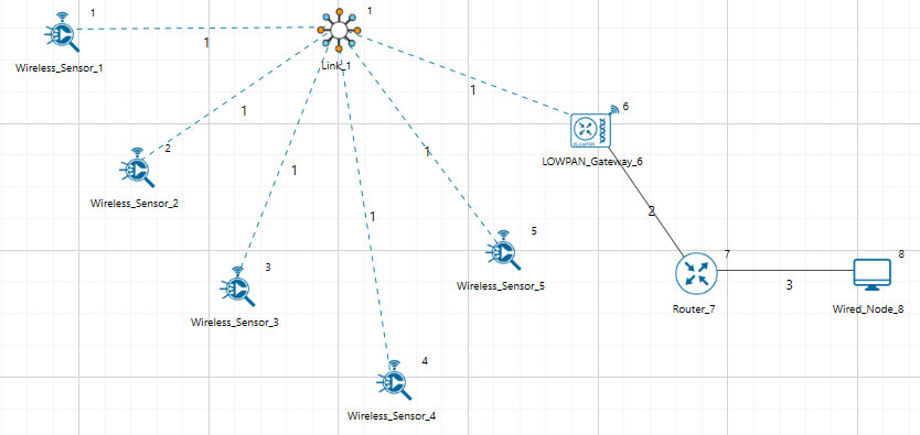
Consider the above scenario as shown in Figure 3-1,
Set pathloss as Log distance with a pathloss exponent of 3.5.
This can be done by clicking on the link, which will open a right-hand panel where you can set the properties as discussed.
Set Grid length as 100\(\times\)100.
Run the simulation for 10s.
Once the simulation is completed, users can access the rpl log file from the results dashboard as shown in Figure 3-2.

However, to get detailed information related to Rank Calculations the DEBUG_RPL preprocessor directive needs to be uncommented in the code.
Procedure to get the RPL log file:
Go to NetSim Home page and click on Your work.
Click on Workspace Options and then click on Open Code and open the codes in Visual Studio. Set x86 or x64 according to the NetSim build which you are using.
Go to the RPL Project in the Solution Explorer. Open RPL.h file and change
// #define DEBUG_RPLto#define DEBUG_RPLas shown below:

Right click on the RPL project in the solution explorer and click on rebuild.
After the RPL project is rebuilt successfully, go back to the network scenario.
Now after any IoT-RPL simulation, an RPL log file is generated with detailed information about the DODAG formation. An example rpl log file is shown below Figure 3-4.

Explanation of the log file:
Step 1:
Node 1 receives a DIO msg from Node 6 (i.e., root).
Node 1 finds the DODAG id.
Based on the DIO message received from Node 6, Node 1 chooses its “Parent as Node 6” and establishes its “New Rank = 13”. It does not have any siblings.

Step 2:
Node 2 receives a DIO msg from Node 6 (i.e. root).
Node 2 finds the DODAG id.
Based on the DIO message received from Node 6, Node 2 chooses its “Parent as Node 6” and establishes its “New Rank = 15”. It does not have any siblings.

Step 3:
Node 6 receives a DAO message from Node 1 with the new route information about the destination and the Gateway.

Step 4:
Node 4 receives a DIO msg from Node 1 (i.e. Sensor which is configured as Router).
Node 4 finds the DODAG id.
Based on the DIO message received from Node 1, Node 4 chooses its “Parent as Node 1” and establishes its “New Rank = 27” since it is in the next Rank level. It does not have any siblings.

Likewise, DODAG formation throughout the simulation is logged inside the rpl log file.
Viewing RPL control messages in Wireshark
Wireshark option can be enabled in the ZigBee devices to capture network traffic during the simulation. RPL control messages such as DAO, DIO etc. can be seen in Wireshark as shown in Figure 3-9.

Following is a screenshot of a DIO message where the Rank information is highlighted as shown in Figure 3-10.

MAC / PHY: 802.15.4 Overview
IEEE802.15/TG4 formulated the IEEE802.15.4 for low-rate wireless personal area network, i.e., LR-WPAN. The standard gives priority to low-power, low-rate and low-cost.
In NetSim, the WSN part of the IOT Network runs 802.15.4 in MAC and PHY. The features implemented are:
PHY rate is fixed at 250 Kbps; it does not vary per the received SNR.
Receive sensitivity is a GUI parameter modifiable by users; the default value is \(-85\) dBm.
Superframe
Beacon enabled and beacon disabled mode.
In beacon enabled mode NetSim supports slotted CSMA/CA with Active & Inactive Period (controlled by Beacon order and super-frame order parameters).
GTS is not implemented.
Data Transfer Model
Device to coordinator, coordinator to device and device to device (peer to peer topology).
AckRequestFlag: If set the device acknowledges successful reception of the data frame by transmitting an ack frame.
Frames
Beacon
Data
Acknowledgement
CSMA / CA Mechanism
Non-beacon mode uses unslotted CSMA/CA.
Beacon mode uses slotted CSMA/CA.
Energy Model
Energy sources: Main Line and Battery.
Energy Harvesting which uses recharging current to replenish battery energy.
Consumption Modes: Transmit, Receive, Idle and Sleep.
CSMA/CA Implementation in NetSim
In both Slotted and Unslotted CSMA/CA cases, the CSMA/CA algorithm is based on backoff periods, where one backoff period is equal to aUnitBackoffPeriod which is 20 symbols long.
This is the basic time unit of the MAC protocol and the access to the channel can only occur at the boundary of the backoff periods. In slotted CSMA/CA the backoff period boundaries must be aligned with the super-frame slot boundaries whereas in unslotted CSMA/CA the backoff periods of one device are completely independent of the backoff periods of any other device in a PAN.
The CSMA/CA mechanism uses three variables to schedule the access to the medium:
NB is the number of times the CSMA/CA algorithm was required to backoff while attempting access to the current channel. This value is initialized to zero before each new transmission attempt.
CW is the contention windows length, which defines the number of backoff periods that need to be clear of channel activity before starting transmission. CW is only used with the slotted CSMA/CA. This value is initialized to 2 before each transmission attempt and reset to 2 each time the channel is assessed to be busy.
BE is the backoff exponent, which is related to how many backoff periods a device must wait before attempting to assess the channel activity.
In beacon-enabled mode, each node employs two system parameters: Beacon order (BO) and Superframe Order (SO).
The parameter BO decides the length of beacon interval (BI), where \(BI= aBaseSuperframeDuration \times {2}^{BO}\) symbols and \(0 \leq BO \leq 14\); while the parameter SO decides the length of superframe duration (SD),
where \(SD = aBaseSuperframeDuration \times {2}^{SO}\) symbols and \(0 \leq SO \leq BO \leq 14\).
The value of aBaseSuperframeDuration is fixed to 960 symbols. The format of the superframe is defined as shown in the following Figure 3-11.

Furthermore, the active portion of each Superframe consists of three parts: beacon, CAP, and CFP, which is divided into 16 equal length slots. The length of one slot is equal to \(aBaseSlotDuration \times {2}^{SO}\) symbols, where aBaseSlotDuration is equal to 60 symbols.
In CAP, each node performs the CSMA/CA algorithm before transmitting data packet or control frame. Each node maintains three parameters: the number of backoffs (NB), contention window (CW), and backoff exponent (BE).
The initial values of NB, CW, and BE are equal to 0, 2, and Min Backoff Expo, respectively, where Min Backoff Expo is by default 3 and it can be set up to 8.
For every backoff period, node takes a delay for random backoff between 0 and \({2}^{BE}-1\) Unit backoff Time (UBT), where UBT is equal to 20 symbols (or 80 bits).
A node performs clear channel assessment (CCA) to make sure whether the channel is idle or busy, when the number of random backoff periods is decreased to 0.
The value of CW will be decreased by one if the channel is idle; and the second CCA will be performed if the value of CW is not equal to 0. If the value of CW is equal to 0, it means that the channel is idle; then the node starts data transmission.
However, if the CCA is busy, the value of CW will be reset to 2; the value of NB is increased by 1; and the value of BE is increased by 1 up to the maximum BE (Max Backoff Expo), where the value Max Backoff Expo is by default 5 and can be up to 8.
The node will repeatedly take random delay if the value of NB is less than the value of Max CSMA BO (macMaxCSMABackoff), where the value of Max CSMA BO is equal to 4; and the transmission attempt fails if the value of NB is greater than the value of Max CSMA BO.
Beacon Order and Superframe Order
Beacon frame is one of the management frames in IEEE 802.15.4 based WSNs and contains all the information about the network. A coordinator in a PAN can optionally bound its channel time using a Superframe structure which is bound by beacon frames and can have an active portion and an inactive portion. The coordinator enters a low-power (sleep) mode during the inactive portion.
The structure of this Superframe is described by the values of macBeaconOrder and macSuperframeOrder. The MAC PIB attribute macBeaconOrder, describes the interval at which the coordinator shall transmit its beacon frames. The value of macBeaconOrder, BO, and the beacon interval, BI, are related as follows:
For \(0\leq BO\leq 14, BI=aBaseSuperframeDuration\times {2}^{BO}\) symbols.
If BO = 15, the coordinator shall not transmit beacon frames except when requested to do so, such as on receipt of a beacon request command. The value of macSuperframeOrder, SO shall be ignored if BO = 15.
If SuperFrame Order (SO) is same as Beacon Order (BO) then there will be no inactive period and the entire SuperFrame can be used for packet transmissions. If BO=10, SO=9 half of the Superframe is inactive and so only half of Superframe duration is available for packet transmission. If BO=10, SO=8 then \({\left(\frac{3}{4}\right)}^{th}\) of the Superframe is inactive and so nodes have only \({\left(\frac{1}{4}\right)}^{th}\) of the Superframe time for transmitting packets.
Energy Models: Sources, Consumption and Harvesting
Wireless nodes, especially sensors, possess limited processing capability, storage and energy resources. The life of the sensor nodes i.e., the energy consumption during its operation, is critical to the network performance. Therefore, researchers often need to study energy consumption at the devices and in the network.
NetSim has dedicated energy models at sensor nodes (WSN/IoT networks) for modelling energy sources, energy consumption and energy harvesting.
The power model is user configurable and can be found in the ZigBee Interface properties of the Sensor nodes as shown in Figure 3-12. The default settings are as per Reference document [1].
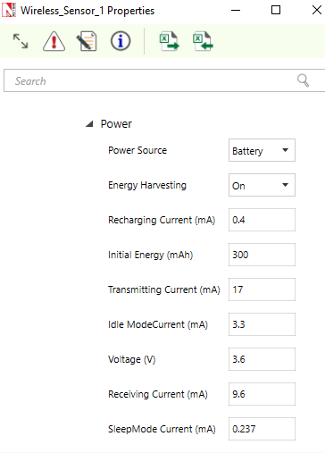
The power source represents the source of energy. Each node has its own single source of power. Main line power source is assumed to have infinite energy while batteries have limited initial energy. When energy harvesting is turned on, it replenishes the battery energy. If the power of a node is completely depleted the node can no longer operate.
NetSim assumes a fixed voltage and the different current drawn in the energy calculations are: Transmit current, \({I}_{t}\), Receive current, \({I}_{R}\), Idle mode current, \({I}_{I}\), and Sleep mode current, \({I}_{S}\). This is a basic energy model and doesn’t take into account battery non-linearities. The energy consumed in each of these activities would be
\[{E}_{TX} = {I}_{t}\cdot V\cdot {T}_{TX}\]
Where \({E}_{TX}\) is the transmit energy, \(V\) is the battery voltage and \({T}_{Tx}\) is the time spent for transmitting packets. And along similar lines
\[{E}_{RX}={I}_{R}\cdot V\cdot {T}_{RX}\]
\[{E}_{I}={I}_{I}\cdot V\cdot {T}_{I}\]
\[{E}_{S}={I}_{S}\cdot V\cdot {T}_{S}\]
And the total energy consumed, \({E}_{cons}\) is given by
\[{E}_{Cons}={E}_{TX}+{E}_{RX}+{E}_{I}+{E}_{S}\]
NetSim also has an Energy-Harvesting Model given by
\[{E}_{EH} = {I}_{RC}\times V\times {T}_{RC}\]
where, \({E}_{EH}\) is the harvested energy, \({I}_{RC}\) is the recharging current and \({T}_{RC}\) is the time for which the battery is recharged. Putting these together we get the expression
\[{E}^{t}={E}_{init}-{E}_{Cons}^{t}+{E}_{EH}^{t}\]
Where \({E}^{t}\) is the energy at time \(t\), \({E}_{Cons}^{t}\) is the energy consumed till time \(t\), \({E}_{EH}^{t}\) is the energy harvested till time \(t\), and \({E}_{init}\) is the initial energy of the battery.
Energy consumption is calculated individually for each sensor node that is part of the network scenario. The sensors have various Radio States such as SLEEP, TRX ON BUSY, RX ON IDLE, RX ON BUSY, RX OFF. As explained in the formulas above the energy consumed is proportional to the time for which the node is in a particular state. For example, the time for which a node transmits a packet is equal to the time for which the node is in TRX ON BUSY state. This duration in turn depends on the protocol operation. Thus, there is a correlation between protocol operation and energy consumption.
The units in NetSim for current is mA, for Voltage is V and for Total-Energy-Consumed is \(mJ\). The Unit for Initial-Energy is \(mAh\) and this is converted to \(mJ\) for calculations since the output metrics are in \(mJ\). The Initial energy in \(mAh\) is converted to \(mJ\) using the formula:
\[{E}_{init}\left[mJ\right]= {E}_{init}\left[mAh\right]\times V\left[V\right]\times 3600\]
For example, if we set \(Initial\ energy=0.5mAh\), and if the voltage in 1V then \({E}_{init}\left[mJ\right]= 1\cdot 0.5\cdot 3600=1800mJ\).
Post simulation NetSim outputs an Energy Metrics table which provides energy consumption of each device with respect to Transmission, Reception, Idle Mode, and Sleep Mode as shown in Figure 3-13.

Energy Model source code
The Energy consumed by the sensor devices are computed in the
function battery_set_mode() present in the BatteryModel.c
file which belongs to the BatteryModel project. This is called in the
function fn_NetSim_Zigbee_ChangeRadioState() present in the
ChangeRadioState.c file which belongs to ZigBee project. The protocol
operations decide the time for which the radio is in a particular state.
The energy calculation function then multiplies this time by the current
drawn and the voltage.
Users can implement energy aware protocols by accessing the information such as remaining energy of each node, when modifying the source code.
Sensor Application and how to model sensing interval
Agents and sensing range were used in earlier versions (before v11) of NetSim as an abstraction of physical phenomenon to trigger packet generation in the sensor nodes respectively. Sensor nodes generate packets whenever they sense an agent within the sensor range. From NetSim v11 onwards users have the facility to configure traffic in the sensor network using the application as shown in Figure 3-14.
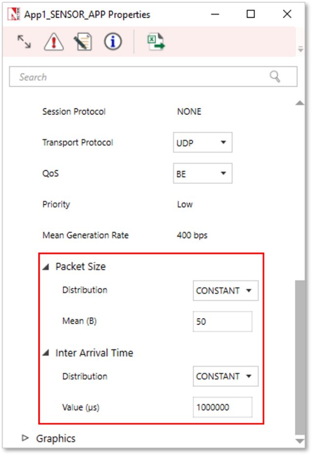
In the application properties, the size of the packet can be set under packet size and the Inter-arrival time can be thought of as sensor interval.
Users can now configure traffic between sensor and sink node as well as between the sensor nodes.
Note that Agents, sensor interval, sensor range are deprecated in NetSim v11.
WSN/IOT File Based Placement
File based placement, as the name suggests is an option that can be used to place devices in user defined locations based on the text file which is provided as the input.
Why do we need File Based Placement
File Based Placement gives a completely user-defined approach for device placements during the process of Network design.
This feature allows the user to design a large network scenario comprising of various devices with ease.
It allows device placements with precision and so on.
Create a text file as per the following or use the file present in
the Docs folder of NetSim Install Directory
< C:\Program Files\NetSim Standard\Docs\Sample Configuration\IOT>
Internet of Things
The text file that we give as an input can be saved as follows: IOT File Based Placement.txt
The general format to be followed while creating an IOT File Based Placement.txt for all the devices used in it is given below:
<DEVICE NAME>,<DEVICE TYPE>,<X>,<Y>
where,
DEVICE NAME represents the name of the device and can be user defined.
DEVICE TYPE represents the type of device, and this info can be obtained from the “General Properties” of that particular device.
X represents the X Coordinate position of the device upon the grid.
Y represents the Y Coordinate position of the device upon the grid.
NOTE: Once we give a file-based input for device placement, an ad-hoc link will automatically be established connecting all the devices pertaining to it. And users need to manually connect the remaining devices using the Wired/Wireless links.
Must the IOT text file contain only IOT devices
The IOT csv file can include all the devices that are present in the top ribbon/toolbar when we select Internet of Things from the home screen. This varies based on the network type. For e.g. WSN and MANETs network types support different devices comparatively.
IOT File based placement.csv
Format: Device_Name,Device_Type,X,Y
Wireless Sensor,Sensors,0,0
Wireless Sensor,Sensors,10,10
Wireless Sensor,Sensors,20,20
Wireless Sensor,Sensors,30,30
Wireless Sensor,Sensors,40,20
Low Pan Gateway,GateWay,50,10
Open NetSim and click New Simulation \(\rightarrow\) Internet Of Things. In the Fast Config window, Choose the File Based Placement option under Automatic Placement and give the path of the text file as shown in Figure 3-15.

After giving the path, Click on OK. It will display the IOT network as shown below, where all devices are placed as per the positions given in the text file.
Connect Low Pan Gateway to Router and Router to Wired node. Configure application and run simulation.
Wireless Sensor Networks
Create a csv file as per the following or use the file present in the
Docs folder of NetSim Install Directory
< C:\Program Files\NetSim Standard\Docs\Sample_Configuration\WSN>
WSN_File_based_placement.csv
Format: Device_Name,Device_Type,X,Y
Wireless_Sensor,Sensors,5,5
Wireless_Sensor,Sensors,10,10
Wireless_Sensor,Sensors,20,10
Wireless_Sensor,Sensors,5,10
WSN_Sink,sinknode,10,15
Open NetSim and click New Simulation \(\rightarrow\) Wireless Sensor Networks. Select File Based Placement option under Automatic Placement and give the path of the text file as shown in Figure 3-17.

After giving the path, Click on OK. It will display the WSN network as shown below, where all devices are placed as per the positions given in the text file.

NOTE: Please refer to section “2.1 Fast configuration” for more information.
Radio measurements log file
NetSim IEEE 802.15.4 Radio Measurements csv log file records pathloss, shadowing loss, fading loss, received power, transmitted power, SNR, BER. This log can be enabled by clicking on configure reports in top ribbon \(\triangleright\) Plots \(\triangleright\) Select IEEE 802.15.4 Radio Measurements under Network Logs as shown below.

The IEEE802.15.4 Radio Measurements log.csv file will contain the following information:
Time in Millisecondss
Transmitter Name
Receiver Name
Distance between the Transmitter and the Receiver in meters
Packet ID
Packet Type
Control Packet Type
Transmitter Power in dBm
Total Loss in dB
Pathloss in dB
Shadowing Loss in dB
Fading Loss in dB
Received Power in dBm
SNR in dB
BER
The log file can be accessed from the Simulations Results Window under the logs as shown below.


Implementation details and Assumptions
The log is written during each packet received at the physical layer (PHY IN). Hence the number of entries will be based on the number of packets received, by all nodes or specific nodes based on values present in the DEVICE ID LIST array.
Energy log file
NetSim Energy log file records Current Time, Mode Switch Time, Mode, Device Name, Device Id, Voltage, Mode Current, Initial Energy, Remaining Energy, Transmit Energy, Receive Energy, Idle Energy, Sleep Energy, Harvested Energy, Consumed Energy.
The Energy log can be enabled by clicking on the icon present in the tool bar as shown below.

The Energy Log.csv file will contain the following information:
Current Time in Milliseconds
Mode Switch Time in Milliseconds
Mode, Current device Mode
Device Name
Device Id
Voltage
Mode Current, Current associated with Mode
Initial Energy in Millijoules
Remaining Energy in Millijoules
Transmit Energy in Millijoules
Receive Energy in Millijoules
Idle Energy in Millijoules
Sleep Energy in Millijoules
Harvested Energy in Millijoules
Consumed Energy in Millijoules
The log file can be accessed from the Simulations Results Window under the log file drop down in the left pane.


Implementation details and Assumptions:
Mode Switch Time indicates the time when the device is set to current Mode.
Mode Current, Current associated with Mode.
Mobility Log File
NetSim mobility log file records Time, Device Name, Device Id, Position X, Position Y, Position Z. The Mobility log can be enabled by clicking on icon present in the tool bar as shown below.

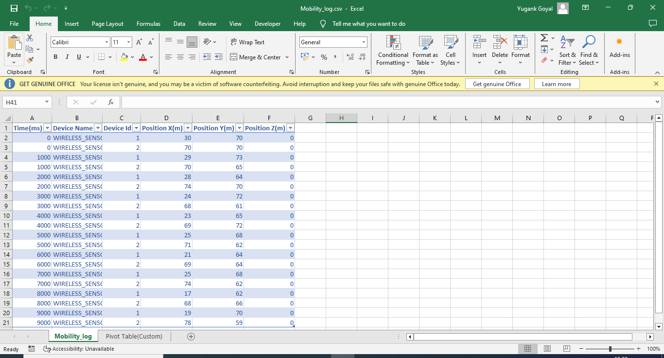
The Mobility Log.csv file will contain the following information:
Time in Milliseconds
Device Name
Device Id
Position X(m)
Position Y(m)
Position Z(m)
The log file can be accessed from the Simulations Results Window under the log file drop down in the left pane.

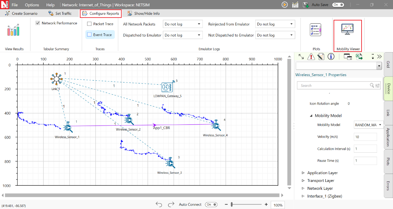
Additionally, the mobility path for sensors can be observed in the design window using mobility viewer option as shown in the screenshot below. For more details on the mobility viewer refer the user manual section 8.6.
Model Limitations
NetSim currently supports only a single root in RPL.
NetSim GUI supports only one RPL instance. Multiple RPL instances can be created by manually editing the config file.
DODAG Repair is not supported.
Nodes (sensors) in NetSim retrieve time from the same (single) virtual clock that ticks virtual time within NetSim. As such, they can be considered as perfectly time synchronized. Real world clocks drift from a reference clock due to various reasons (heat, deficient oscillator, etc.,), resulting in an offset of a few milliseconds per day. In the COTS version of NetSim, clock drift is not available. This means that it is not possible to model clocks to run with different rates and/or offsets, in different nodes/sensors.
Security in 802.15.4 is not implemented.