Satellite Antenna Pattern
In the section above the link budgets were calculated assuming the max transmit antenna gain. However, per section 6.4.1 of TR 38.811, we know that the normalized antenna gain pattern, corresponding to a typical reflector antenna with a circular aperture, is given by
\[\begin{array}{ll} 1 & for\;\theta = 0 \\[10pt] 4\left|\dfrac{J_1(ka\sin\theta)}{ka\sin\theta}\right|^2 & for\;0 < |\theta| \leq 90^{\circ} \end{array}\]
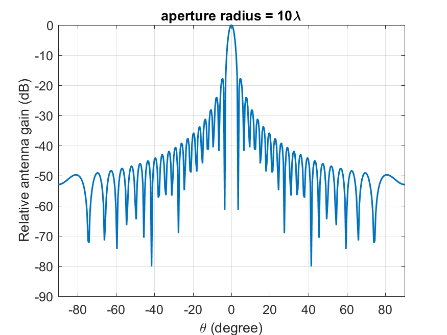
where \(J_1(x)\) is the Bessel function of the first kind and first order with argument \(x\), \(a\) is the radius of the antenna’s circular aperture, \(k =\frac{2\pi f}{c}\) is the wave number, \(f\) is the frequency of operation, \(c\) is the speed of light in a vacuum and \(\theta\) is the angle measured from the boresight of the antenna’s main beam. Note that \(ka\) equals the number of wavelengths on the circumference of the aperture and is independent of the operating frequency. The above expression provides the gain in linear scale and it needs to be converted to dB scale. The normalized gain pattern for \(a = 10\frac{c}{f}\) (aperture radius of 10 wavelengths) is shown below
Off Boresight Angle Calculation
Conceptually, the off-boresight angle, \(\theta\), in the antenna gain formula is defined as the angle between two vectors: one along the boresight of the beam (i.e., from the satellite to the beam centre, which corresponds to the sub-satellite nadir point), and the other from the satellite to the UE. In NetSim \(\theta\)is computed as the arccosine of the normalized dot product of these two vectors.
Standard ENU-Based Look Angle Computation (Satellite to Earth)
This section describes the standard ENU (East–North–Up) method for computing satellite look angles (azimuth and elevation) as seen from an earth station (user terminal).
Notation
\(\varphi_{t}\) : Latitude of earth station (degrees)
\(\lambda_{t}\) : Longitude of earth station (degrees)
\(H_{t}\) : Altitude of earth station above sea level (km)
\(\varphi_{s}\) : Latitude of satellite (degrees)
\(\lambda_{s}\) : Longitude of satellite (degrees)
\(H_{s}\) : Altitude of satellite above sea level (km)
Step 1: Convert Geodetic Coordinates to ECEF
Convert both earth station and satellite geodetic coordinates to Earth-Centered Earth-Fixed (ECEF) Cartesian coordinates.
WGS-84 ellipsoid constants
WGS-84 defines the Earth as an oblate ellipsoid with:
Semi-major axis (equatorial radius):
\[\begin{equation} a = 6378137.0 \text{ m} \end{equation}\]
Flattening:
\[\begin{equation} f = \frac{1}{298.257223563} \end{equation}\]
First eccentricity squared:
\[\begin{equation} e^{2}=2f-f^{2} \end{equation}\]
Numerically:
\[\begin{equation} e^{2} \approx 0.00669437999014 \end{equation}\]
Prime vertical radius of curvature
\[\begin{equation} N(\phi) = \frac{a}{\sqrt{1 - e^{2}\sin^{2}(\phi)}} \end{equation}\]
This is to compensate for Earth’s flattening.
ECEF Conversion formulas (WGS-84)
\[\begin{equation} X = (N + h)\cos(\phi)\cos(\lambda ) \end{equation}\]
\[\begin{equation} Y = (N + h)\cos(\phi)\sin(\lambda ) \end{equation}\]
\[\begin{equation} Z = N\left((1 - e^{2}) + h\right)\sin(\phi) \end{equation}\]
This gives Earth-Centered Earth-Fixed (ECEF) coordinates:
X axis: intersection of equator and Greenwich meridian
Y axis: \(90^{\circ}\) east on equator
Z axis: North pole
Step 2: Line-of-Sight Vector in ECEF
Compute the line-of-sight (LOS) vector from the earth station to the satellite:
\[\begin{equation} \Delta r = r_{s} - r_{t} = (\Delta X, \Delta Y, \Delta Z) \end{equation}\]
Step 3: Rotate LOS Vector into Local ENU Frame
Define the standard ECEF-to-ENU rotation matrix at the earth station latitude \(\varphi_{t}\)and longitude \(\lambda_{t}\):
\[\begin{equation} \begin{bmatrix} E \\ N \\ U \end{bmatrix} = \begin{bmatrix} -\sin(\lambda_{t}) & \cos(\lambda_{t}) & 0 \\ -\sin(\phi_{t}) \cos(\lambda_{t}) & -\sin(\phi_{t}) \sin(\lambda_{t}) & \cos(\phi_{t}) \\ \cos(\phi_{t}) \cos(\lambda_{t}) & \cos(\phi_{t}) \sin(\lambda_{t}) & \sin(\phi_{t}) \end{bmatrix}\begin{bmatrix} \Delta X \\ \Delta Y \\ \Delta Z \end{bmatrix} \end{equation}\]
This yields the local ENU components (E, N, U) of the satellite relative to the earth station.
Step 4: Slant Range
The straight-line distance between the earth station and the satellite is:
\[\begin{equation} D_{ts}= \sqrt{E^{2}+ N^{2}+ U^{2}} \end{equation}\]
Step 5: Elevation Angle
The elevation angle (above the local horizontal plane) is computed as:
\[\begin{equation} el = \text{atan2}\left(U, \sqrt{E^{2}+ N^{2}}\right) \end{equation}\]
Elevation is in the range \(-90^{\circ}\) to \(+90^{\circ}\).
Step 6: Azimuth Angle
The azimuth angle, measured clockwise from true North, is:
\[\begin{equation} az = \text{atan2}(E, N) \end{equation}\]
The result should be wrapped to the range \(0^{\circ}\)–\(360^{\circ}\).
Step 7: Visibility Check
Given a minimum elevation mask angle (maskAngle):
\[\begin{equation} \text{visible} = 1 \quad \text{if } el \geq \text{maskAngle} \end{equation}\]
\[\begin{equation} \text{visible} = 0 \quad \text{otherwise} \end{equation}\]
If \(\sqrt{E^{2}+ N^{2}} \approx 0\)(satellite directly overhead), the azimuth is indeterminate.
Link Budget Calculations: Example 3 LEO 600 and LEO 1200
For the same two examples, shown earlier, if we compute the angular antenna gain based on the UE and satellite positions
Case 1:
\[\begin{equation} f=2.18 \text{ GHz} ;\; a=1 \text{ m} ;\; k=\frac{2\pi f}{c}=\frac{2\times 3.14\times 2.18\times 10^{9}}{3\times 10^{8}}=45.76 \end{equation}\]
The UE associates with beam 3, and the angle between the antenna boresight to the line joining the UE and the satellite is \(\theta =3.33^{\circ}\). This computation is carried out within NetSim. Substituting
\[\begin{equation} 4\left|\frac{J_{1}\left(45.76\times 1\times \sin(3.33)\right)}{45.76\times 1\times \sin(3.33)}\right|^{2}= 4\left|\frac{J_{1}\left(2.656\right)}{2.656}\right|^{2}=0.117 \text{ mW}= -9.31 \text{ dBm} \end{equation}\]
Case 2:
\[\begin{equation} \theta =6.15^{\circ} \end{equation}\]
\[\begin{equation} 4\left|\frac{J_{1}\left(45.76\times 1\times \sin(6.15)\right)}{45.76\times 1\times \sin(6.15)}\right|^{2}= 4\left|\frac{J_{1}\left(4.900\right)}{4.900}\right|^{2}=0.0165 \text{ mW}= -17.82 \text{ dBm} \end{equation}\]
Since EIRP includes the antenna gains, the angular gain values obtained above need to be added in the CNR calculations. The final link budget calculations are shown below. The changes as compared to the earlier table are shown in blue.
| Simulation Parameters | LEO 600 km | LEO 1200 km |
|---|---|---|
| Antenna Aperture (m) | 1 | 1 |
| Beam Radius (Km) | 55.13 | 110.24 |
| EIRP density (dBW/MHz) | 34 | 40 |
| Bandwidth B | 30 | 30 |
| EIRP (dBW) | 48.77 | 54.77 |
| Elevation angle | 80.58 | 85.26 |
| Angular Antenna Gain, \(G(\theta)\), (dB) (Calculation provided above) |
\(-\)9.31 | \(-\)17.82 |
| Slant range d (Km) | 607.48 | 1203.46 |
| Free space pathloss (dB), \(PL_{FS}\) | 154.91 | 160.85 |
| Shadow loss (dB), \(PL_{SM}\) | 0.39 | 0.96 |
| Additional Loss(dB), \(PL_{AD}\) | 2 | 2 |
| Total Pathloss, L(dB) | 157.3 | 163.81 |
| Rx Antenna Gain | 0 | 0 |
| Noise figure f | 7 | 7 |
| Rx Antenna Temp Ta (K) | 290 | 290 |
| RX equivalent antenna Temp, \(T\) [\(dBK\)] | 31.62 | 31.62 |
| Receiver G/T | \(-\)31.62 | \(-\)31.62 |
| Boltzmann constant \(k\) \(\left[\frac{dBW}{\frac{K}{Hz}}\right]\) | \(-\)228.6 | \(-\)228.6 |
| CNR (Calculation provided below) |
4.36 | \(-\)4.66 |
Case 1:
\[\begin{equation} CNR=EIRP+G\!\left(\theta \right)+ Rx\frac{G}{T}-k-PL_{FS}-PL_{SM}-PL_{AD}-B \end{equation}\]
Substituting we get
\[\begin{equation} CNR= 48.77+\left(-9.87\right)+\left(-31.62\right)-\left(-228.6\right)-154.14-0.57-8-74.77=-1.6 \text{ dB} \end{equation}\]
Case 2:
\[\begin{equation} CNR=EIRP+G\!\left(\theta \right)+Rx\frac{G}{T}-k-PL_{FS}-PL_{SM}-PL_{AD}-B \end{equation}\]
Substituting we get
\[\begin{equation} CNR= 54.77+\left(-12.95\right)+\left(-31.62 \right)-\left(-228.6\right)-160.08-0.57-8-74.77=-4.62 \text{ dB} \end{equation}\]