Featured Examples
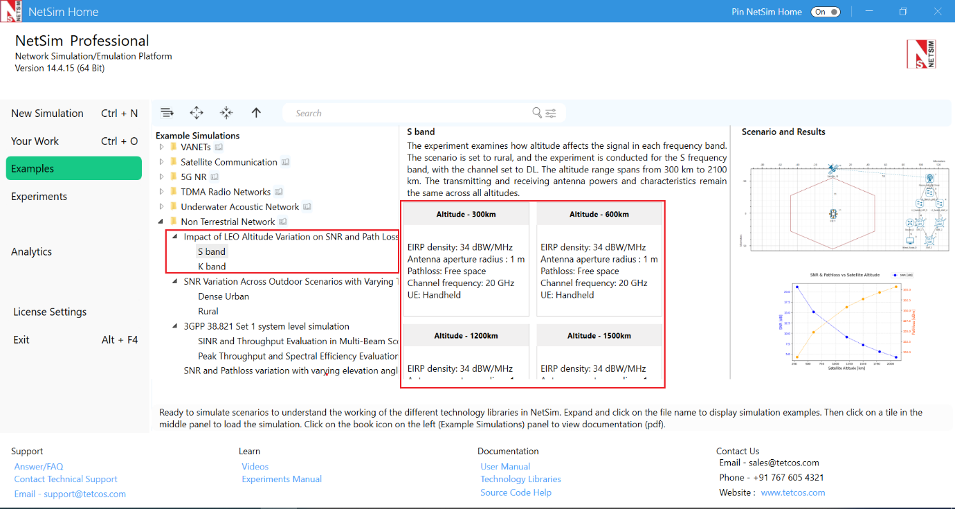
Impact of LEO Altitude Variation on SNR and Path Loss
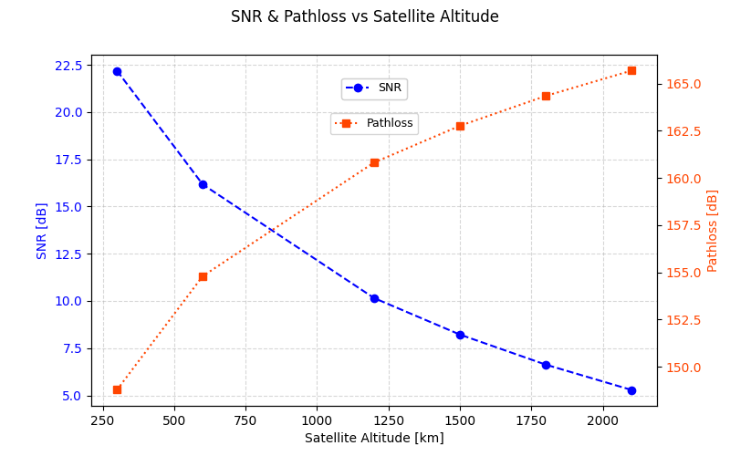
The experiment examines how altitude affects signal in each frequency band. The scenario is set to rural. The experiment is run for two frequency bands of interest (S and K), with the channel set to DL. The altitude range spans from 300km to 2100km. Transmitting and receiving antenna powers and characteristics are the same for each altitude.
To simulate this example in NetSim, Open NetSim, Select Examples \(\triangleright\) Non Terrestrial Network \(\triangleright\) Impact of LEO Altitude Variation on SNR and Path Loss then click on the tile in the middle panel to load the example as shown in below screenshot.
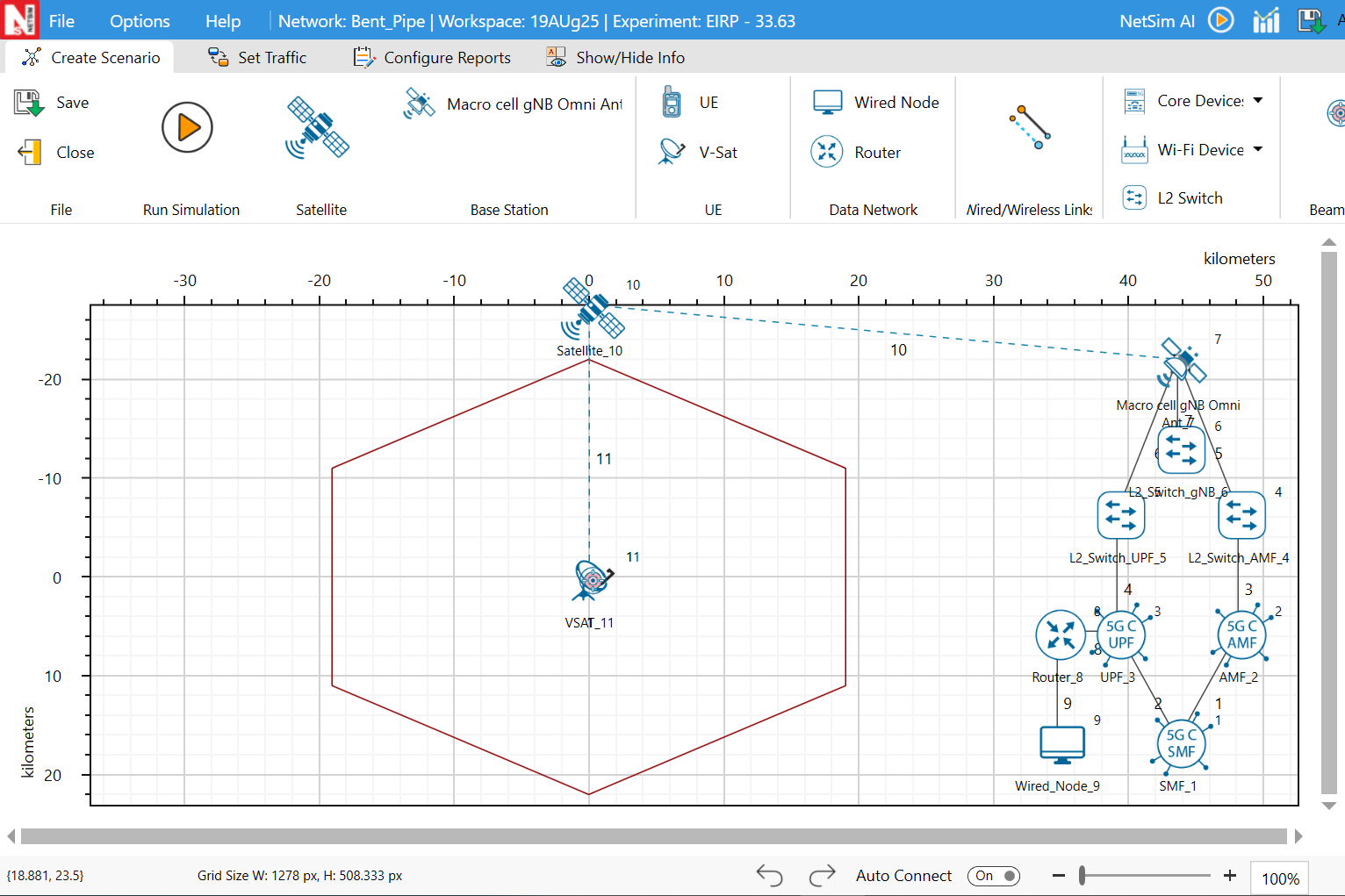
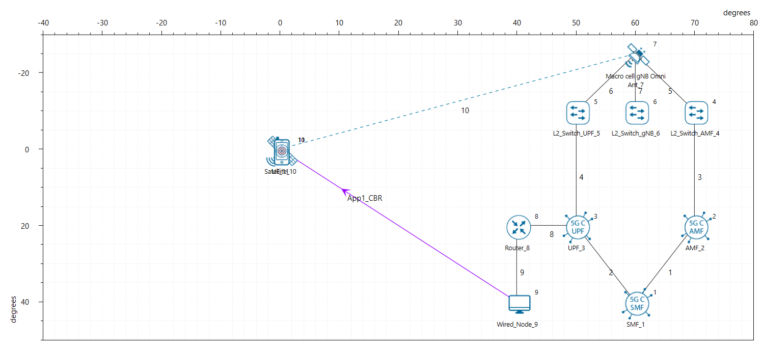
The following network diagram illustrates what the NetSim UI displays when you open the example configuration file.
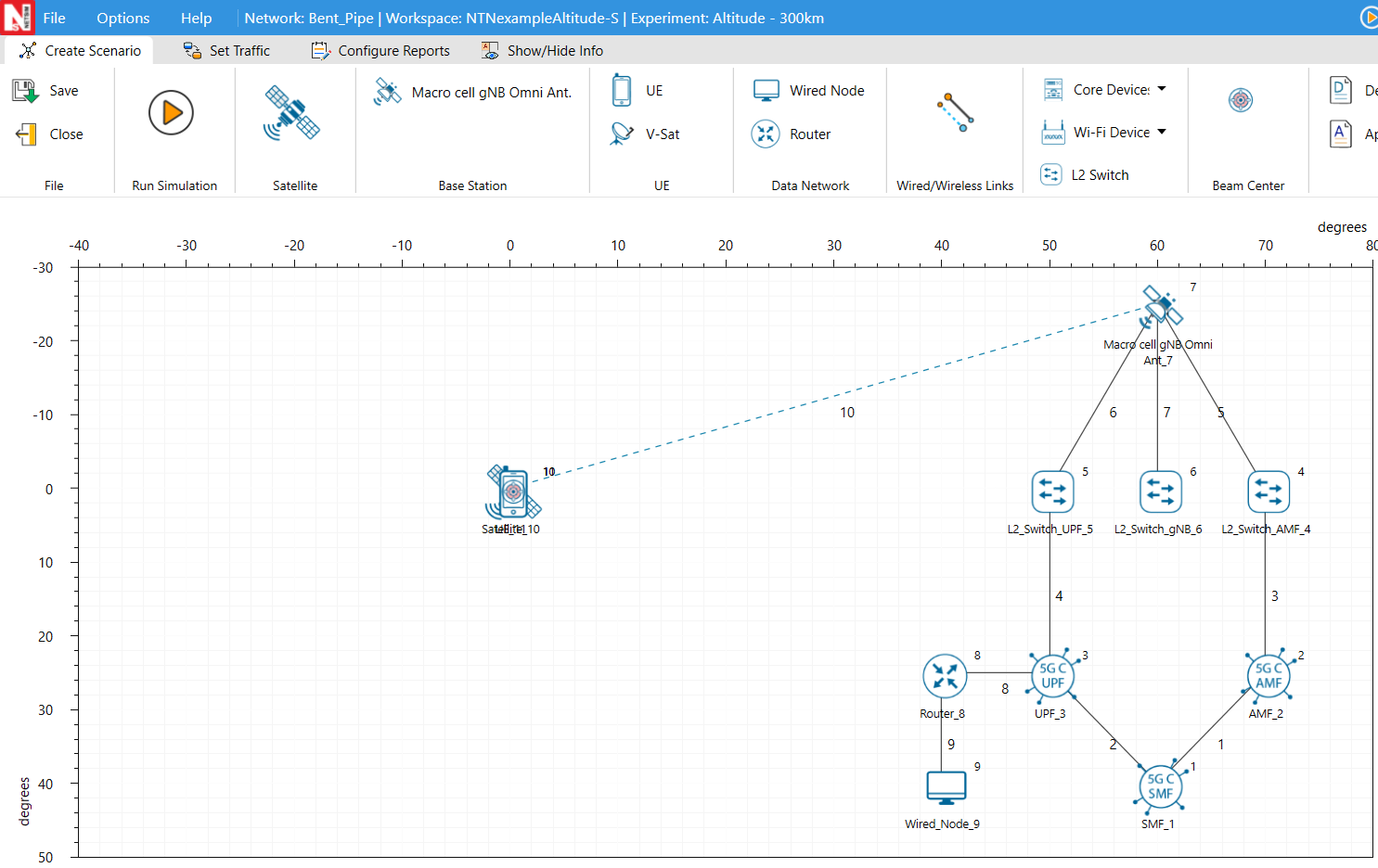
Settings done in example config file for S band
Set the satellite properties as follows. To configure, click on Satellite. On the right side, expand the property panel, go to the Physical Layer of Interface_2 (Service Link), and set the following properties:
| Simulation Properties | Values |
|---|---|
| Satellite \(\triangleright\) Interface_2 (Service link) properties | |
| EIRP Density (dBW/MHz) | 34 |
| Antenna Aperture Radius (m) | 1 |
| Pathloss (dBm) | Free Space |
| Additional Loss (dB) | 0 |
| Shadow Model | None |
| Outdoor Model | Rural |
| Altitude (km) | 300, 600, 1200, 1500, 1800, 2100 |
| UE Noise Figure (dB) | 7 |
| gNB \(\triangleright\) Interface_4 (Feeder link) properties | |
| CA Configuration | S Band n256 |
| Central Frequency (GHz) | 2.185 |
| Channel Bandwidth (MHz) | 20 |
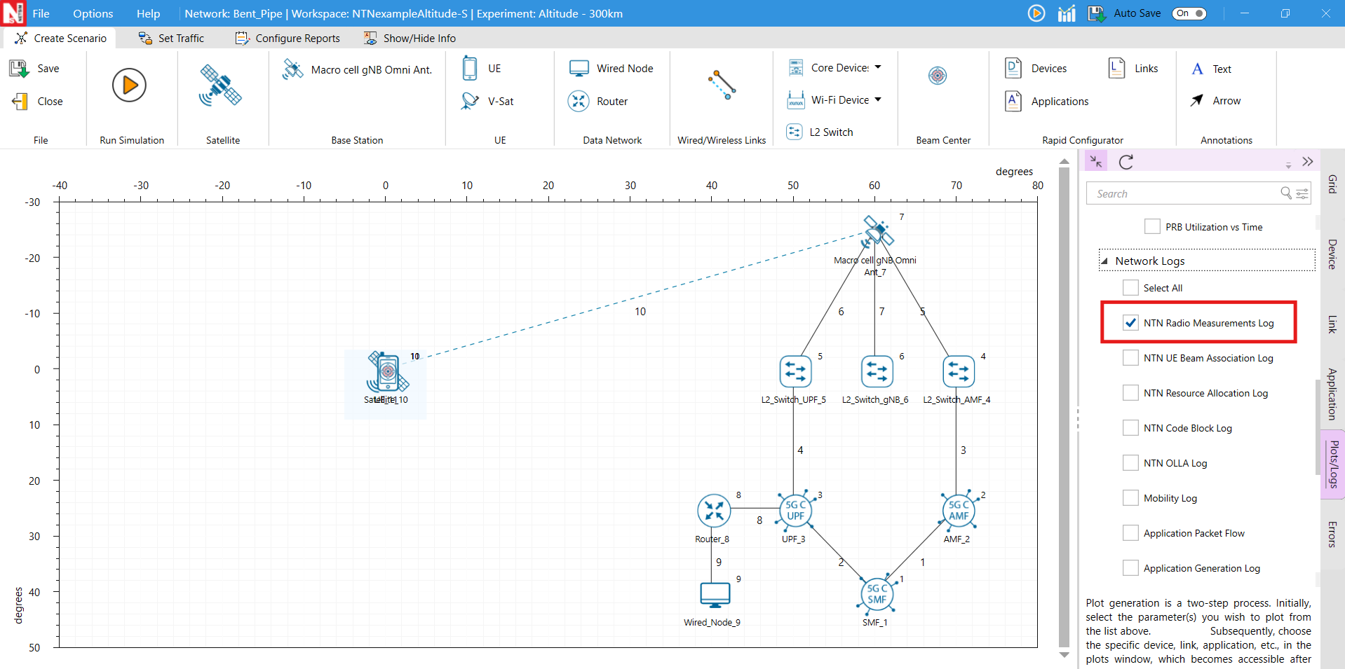
Enable NTN UE Beam association log by clicking on plots/logs tab on the right side of the panel.
Pathloss and SINR calculation for 600 km
We consider the satellite co-ordinates as \((0, 0)\) degree and 600 km altitude, and the UE co-ordinates as \(\left(0, 0\right)\)degree. The elevation angle is calculated as:
\[\begin{equation} \alpha =\sin^{-1}\!\left(\frac{D}{Ru \times L}\right) =90^{\circ} \end{equation}\]
Where,
\[\begin{equation} Ru = \sqrt{x_{ue}^{2} + y_{ue}^{2} + z_{ue}^{2}} \end{equation}\]
\[\begin{equation} L = \sqrt{\left(x_{sat} - x_{ue}\right)^{2} + \left(y_{sat} - y_{ue}\right)^{2} + \left(z_{sat} - z_{ue}\right)^{2}} \end{equation}\]
\[\begin{equation} D = \sqrt{\left(x_{sat} - x_{ue}\right)\cdot x_{ue} + \left(y_{sat} - y_{ue}\right)\cdot y_{ue} + \left(z_{sat} - z_{ue}\right)\cdot z_{ue}} \end{equation}\]
The slant height used in NetSim is per 38.811, equation 6.6-3, i.e.
\[\begin{equation} d=\sqrt{R_{E}^{2}\sin^{2}\!\left(\alpha \right)+h_{o}^{2}+2h_{o}R_{E}}-R_{E}\sin\!\left(\alpha \right) \end{equation}\]
For a link between a ground station and a LEO satellite operating at 600 km with elevation angle \(\alpha =90^{\circ}\).
\[\begin{multline} d=\sqrt{\left(6.371\cdot 10^{6}\right)^{2}\cdot \sin^{2}\!\left(90^{\circ}\right)+\left(6\cdot 10^{5}\right)^{2}+2\cdot \left(6\cdot 10^{5}\right)\left(6.371\cdot 10^{6}\right)}\\ -6.371\cdot 10^{6}\sin\!\left(90^{\circ}\right) \end{multline}\]
\[\begin{equation} d=600 \text{ km} \end{equation}\]
The free space pathloss \(PL_{FS}\) for a channel with \(f_{c}=2.185\) GHz, or \(\lambda =\frac{c}{f}=0.15\) m, and \(d=600\) km is
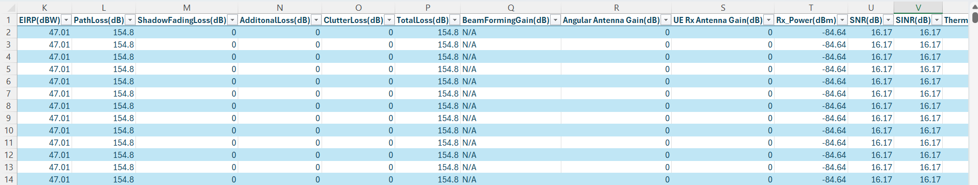
\[\begin{multline} PL_{FS}=20\log_{10}\!\left(\frac{4\pi d}{\lambda }\right)=20\log_{10}\!\left(\frac{4\pi \left(600\times 10^{3}\right)\left(2.185\times 10^{9}\right)}{3\times 10^{8}}\right)=154.8 \text{ dB} \end{multline}\]
\[\begin{equation} CNR=EIRP+G_{Tx}+Rx\frac{G}{T}-k-PL_{FS}-PL_{SM}-PL_{AD}-B \end{equation}\]
\[\begin{equation} CNR=47.01+0+\left(-31.62\right)-\left(-228.6\right)-\left(154.8\right)-0-73.01 \end{equation}\]
\[\begin{equation} =16.17 \text{ dB} \end{equation}\]
Results
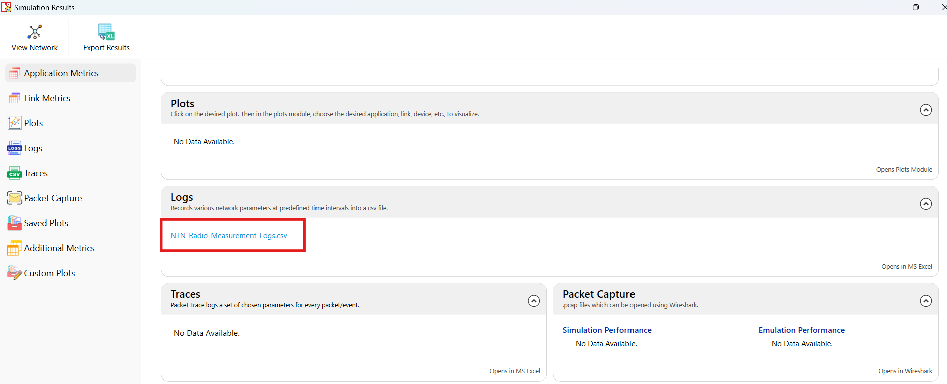
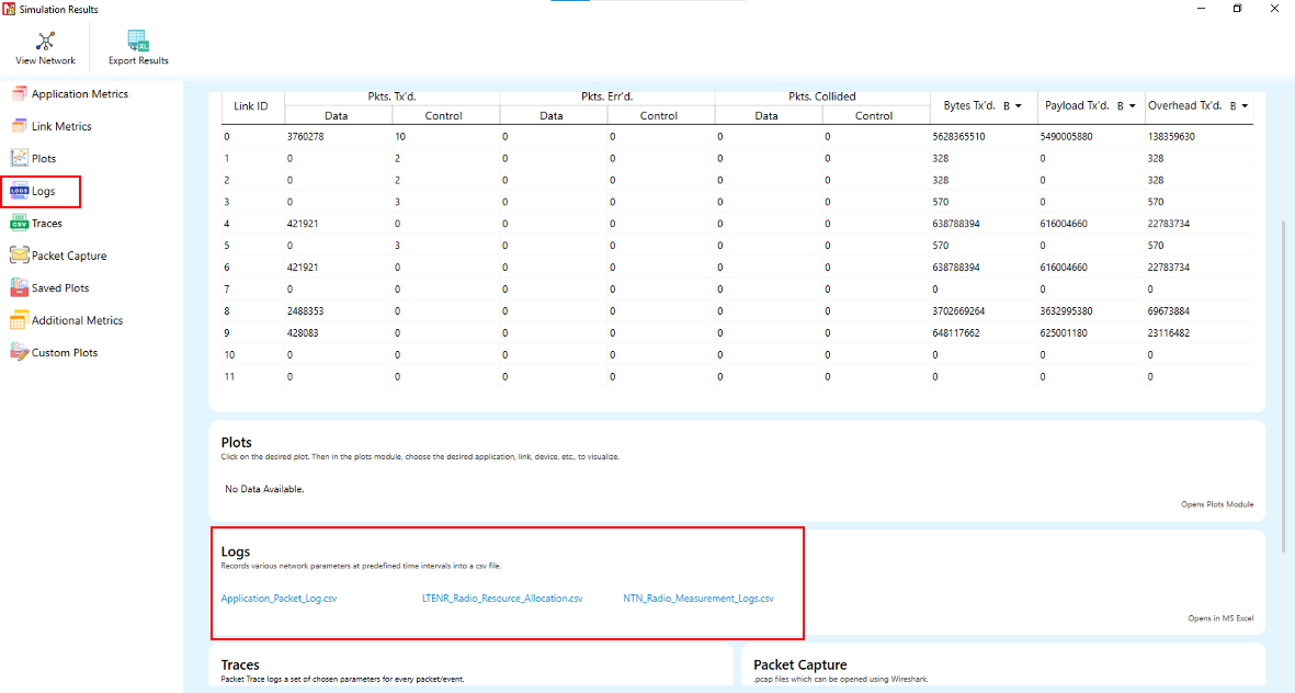
After the simulation, open the NTN UE Radio Measurement.csv under logs section from simulation results window and observe the SNR and pathloss value.
Settings done in example config file for K band
Set the satellite properties as follows. To configure, click on Satellite. On the right side, expand the property panel, go to the Physical Layer of Interface_2 (Service Link), and set the following properties:
| Simulation Properties | Values |
|---|---|
| Satellite \(\triangleright\) Interface_2 (Service link) properties | |
| EIRP Density (dBW/MHz) | 4 |
| Antenna Aperture Radius (m) | 0.25 |
| Pathloss Model | Free Space |
| Additional Loss (dB) | 0 |
| Shadow Fading | None |
| Outdoor Model | Rural |
| Altitude | 300, 600, 1200, 1500, 1800, 2100 |
| VSAT \(\triangleright\) Interface_1 (Service Link) properties | |
| UE Noise Figure (dB) | 1.2 |
| Tx/Rx Antenna Gain (dB) | 35 |
| gNB \(\triangleright\) Interface_4 (Feeder link) properties | |
| CA Configuration | K Band n510 |
| Channel Frequency (GHz) | 18.75 |
| Channel Bandwidth (MHz) | 200 |
Enable NTN UE Beam association log by clicking on plots/logs tab on the right side of the panel.
Run simulation for 10 seconds.
We consider the satellite co-ordinates as \((0, 0)\) degree and 600 km altitude, and the UE co-ordinates as \(\left(0, 0\right)\)degree. The elevation angle is calculated as:
\[\begin{equation} \alpha =\sin^{-1}\!\left(\frac{D}{Ru \times L}\right) =90^{\circ} \end{equation}\]
Where,
\[\begin{equation} Ru = \sqrt{x_{ue}^{2} + y_{ue}^{2} + z_{ue}^{2}} \end{equation}\]
\[\begin{equation} L = \sqrt{\left(x_{sat} - x_{ue}\right)^{2} + \left(y_{sat} - y_{ue}\right)^{2} + \left(z_{sat} - z_{ue}\right)^{2}} \end{equation}\]
\[\begin{equation} D = \sqrt{\left(x_{sat} - x_{ue}\right)\cdot x_{ue} + \left(y_{sat} - y_{ue}\right)\cdot y_{ue} + \left(z_{sat} - z_{ue}\right)\cdot z_{ue}} \end{equation}\]
The slant height used in NetSim is per 38.811, equation 6.6-3, i.e.
\[\begin{equation} d=\sqrt{R_{E}^{2}\sin^{2}\!\left(\alpha \right)+h_{o}^{2}+2h_{o}R_{E}}-R_{E}\sin\!\left(\alpha \right) \end{equation}\]
For a link between a ground station and a LEO satellite operating at 600 km with elevation angle \(\alpha =90^{\circ}\).
\[\begin{multline} d=\sqrt{\left(6.371\cdot 10^{6}\right)^{2}\cdot \sin^{2}\!\left(90^{\circ}\right)+\left(6\cdot 10^{5}\right)^{2}+2\cdot \left(6\cdot 10^{5}\right)\left(6.371\cdot 10^{6}\right)}\\ -6.371\cdot 10^{6}\sin\!\left(90^{\circ}\right) \end{multline}\]
\[\begin{equation} d=600 \text{ km} \end{equation}\]
The free space pathloss \(PL_{FS}\) for a channel with \(f_{c}=18.75\) GHz, or \(\lambda =\frac{c}{f}=0.016\) m, and \(d=600\) km is
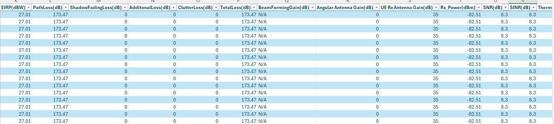
\[\begin{multline} PL_{FS}=20\log_{10}\!\left(\frac{4\pi d}{\lambda }\right)=20\log_{10}\!\left(\frac{4\pi \left(600\times 10^{3}\right)\left(20\times 10^{9}\right)}{3\times 10^{8}}\right)=173.47 \text{ dB} \end{multline}\]
\[\begin{equation} CNR=EIRP+G_{Tx}+Rx\frac{G}{T}-k-PL_{FS}-PL_{SM}-PL_{AD}-B \end{equation}\]
\[\begin{equation} CNR=27.01+0+9.17-\left(-228.6\right)-\left(173.47 \right)-2-83.01 \end{equation}\]
\[\begin{equation} =8.3 \text{ dB} \end{equation}\]
Observe the SNR and pathloss value from NTN UE radio measurement log.
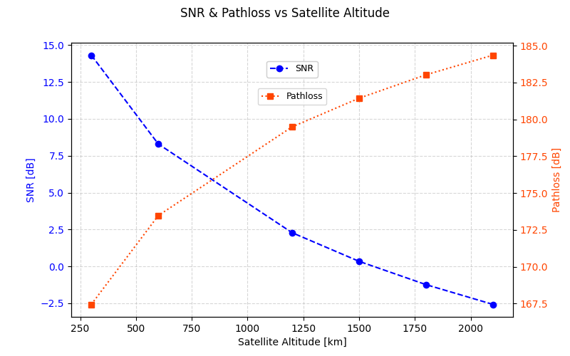
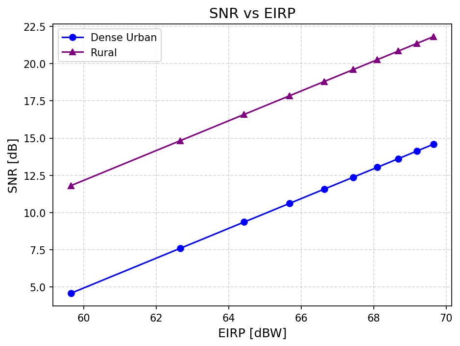
The Ka band, which operates at higher frequencies, experiences greater path loss as can be seen from the example numerical calculation provided. In downlink transmissions, the SNR values for the S-band and K-band cases are comparable. Although the K-band scenario has higher path loss and lower EIRP input, the use of V-SAT antennas with a receiver gain of 35 dBi compensates for these effects, whereas the S-band scenario uses simulated handheld UEs with nil receiver gain.
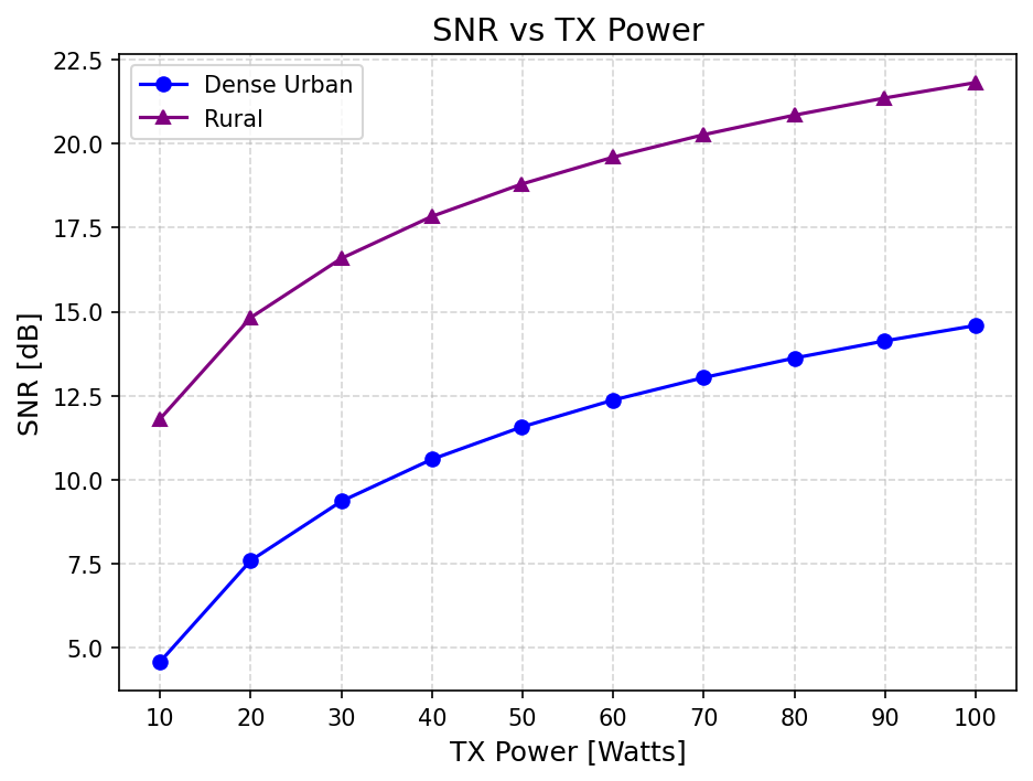
SNR Variation Across Outdoor Scenarios with Varying Transmit Power
To simulate this example in NetSim, Open NetSim, Select Examples \(\triangleright\) Non Terrestrial Network \(\triangleright\) SNR Variation Across Outdoor Scenarios with Varying Transmit Power then click on the tile in the middle panel to load the example as shown in below screenshot.

The following network diagram illustrates what the NetSim UI displays when you open the example configuration file
Settings done in example config file for Dense urban and Rural scenarios
Set the satellite properties as follows. To configure, click on Satellite. On the right side, expand the property panel, go to the Physical Layer of Interface_2 (Service Link), and set the following properties:
| Simulation Properties | Values |
|---|---|
| Satellite \(\triangleright\) Interface_2 (Service link) properties | |
| Antenna Aperture Radius (m) | 1.5 |
| Pathloss Model | Free Space |
| Shadow model | Log Normal |
| Additional Loss(dB) | 0 |
| LOS probability | 0 (NLOS) |
| Clutterloss Model | TR38.811 |
| EIRP Density (dBW/MHz) | 33.63, 36.64, 38.40, 39.65, 40.61, 41.41, 42.08, 42.66, 43.17, 43.63 |
| Tx Power (dBm) | 40.00, 43.01, 44.77, 46.02, 46.98, 47.78, 48.45, 49.03, 49.54, 50.00 |
| VSAT \(\triangleright\) Interface_1 (Service Link) properties | |
| UE Noise Figure (dB) | 1.2 |
| Tx/Rx Antenna Gain (dB) | 35 |
| gNB \(\triangleright\) Interface_4 (Feeder link) properties | |
| CA Configuration | K Band n510 |
| Channel Frequency (GHz) | 18.75 |
| Channel Bandwidth (MHz) | 400 |
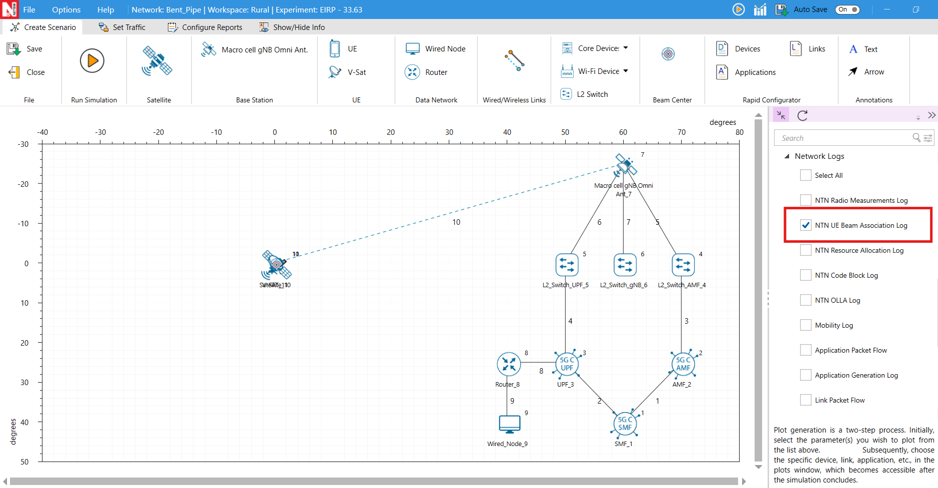
Enable NTN UE Beam association log by clicking on plots/logs tab on the right side of the panel.
Run Simulation for 10 seconds.
Results
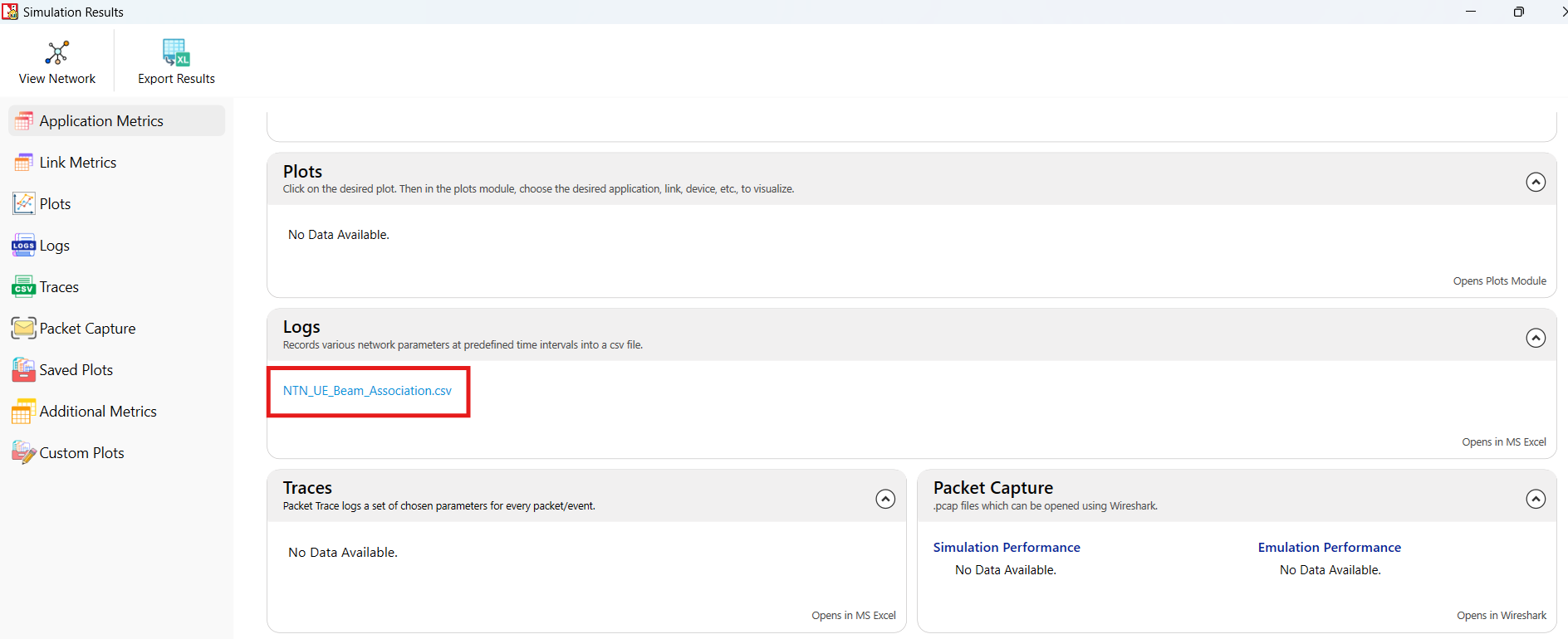
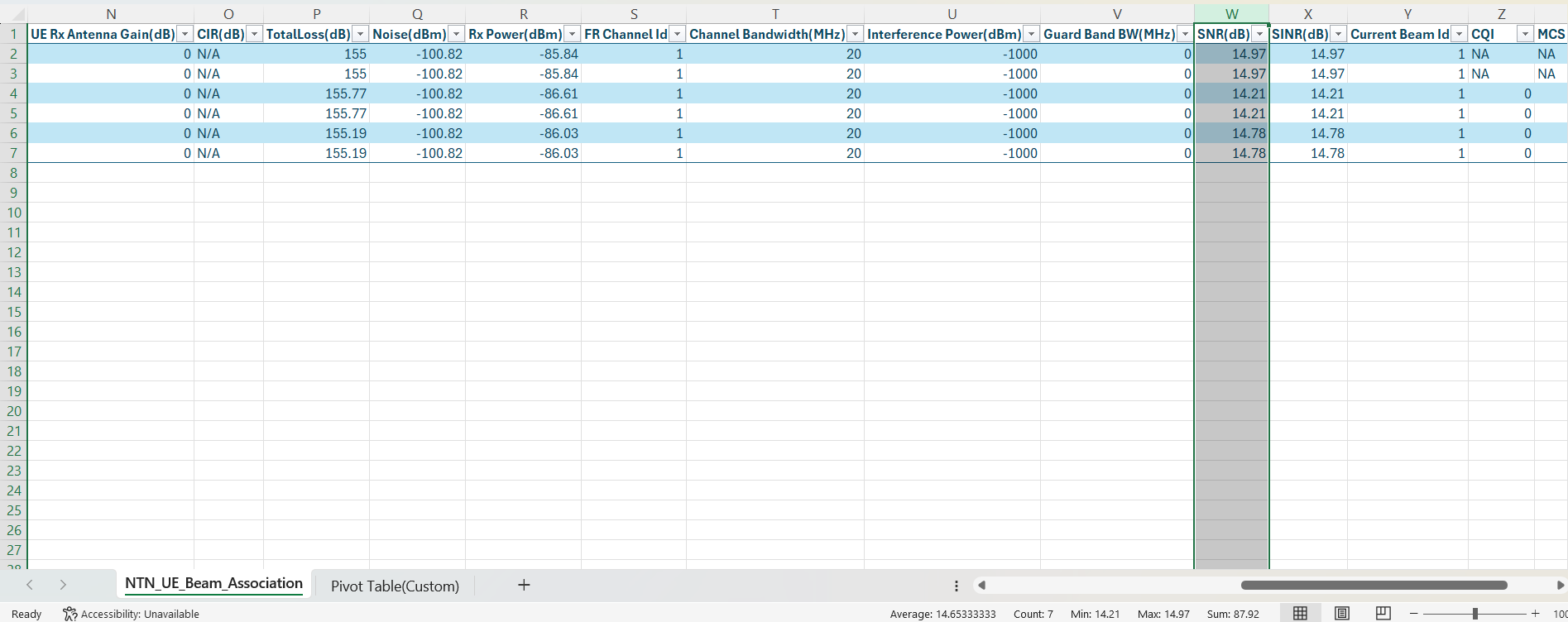
After the simulation, open the NTN UE Beam Association.csv under logs section from simulation results window and observe the SNR value.

Clutter loss enabled and NLOS
If we consider 49.65 as Tx antenna gain, and calculate the Tx power based on that,
\[\begin{equation} EIRP \;[\text{dBW}]= P_{tx}\;[\text{dBm}]-30+G_{Tx}\;[\text{dBi}] \end{equation}\]
\[\begin{equation} 59.65= P_{tx}\;[\text{dBm}]-30+49.65 \end{equation}\]
\[\begin{equation} P_{tx}\;[\text{dBm}]=40 \end{equation}\]
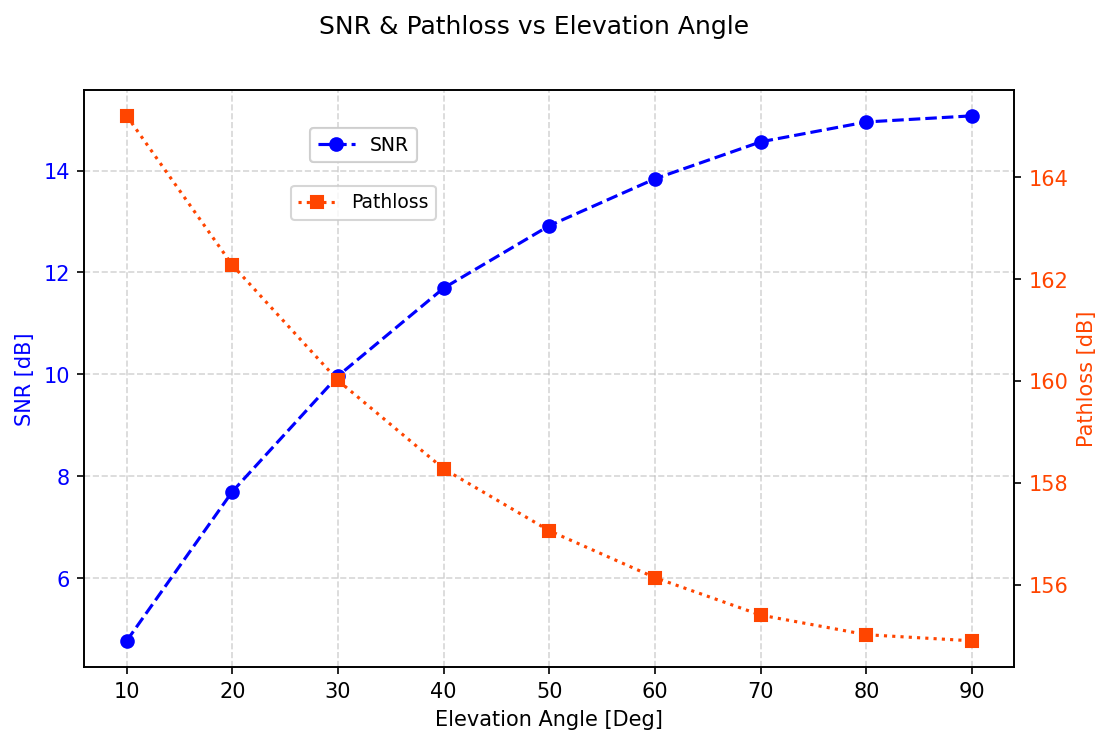
SNR and Pathloss variation with varying elevation angles
In this experiment, a satellite at an altitude of 600km is deployed to measure pathloss and SNR values for different elevation angles. Changing the UE position, but keeping its altitude from ground fixed, aims at simulating how the signal might be affected as a UE moves towards the beam center. The test is performed in DL on the S band. The simulations are performed for every scenario. The results show how dramatically the elevation angle affects the signal, with SNR values that experience an immediate degradation when going from communicating with a satellite that is perfectly positioned to one that is slightly shifted. Elevation angle however, is not the only factor that changes, since the altitude from ground of the satellite is kept the same throughout the test, the distance between the communicating nodes is increasing with the diminishing of the elevation angle.
To simulate this example in NetSim, Open NetSim, Select Examples \(\triangleright\) Non-Terrestrial Network \(\triangleright\) SNR and Pathloss variation with varying elevation angles then click on the tile in the middle panel to load the example as shown in below screenshot.
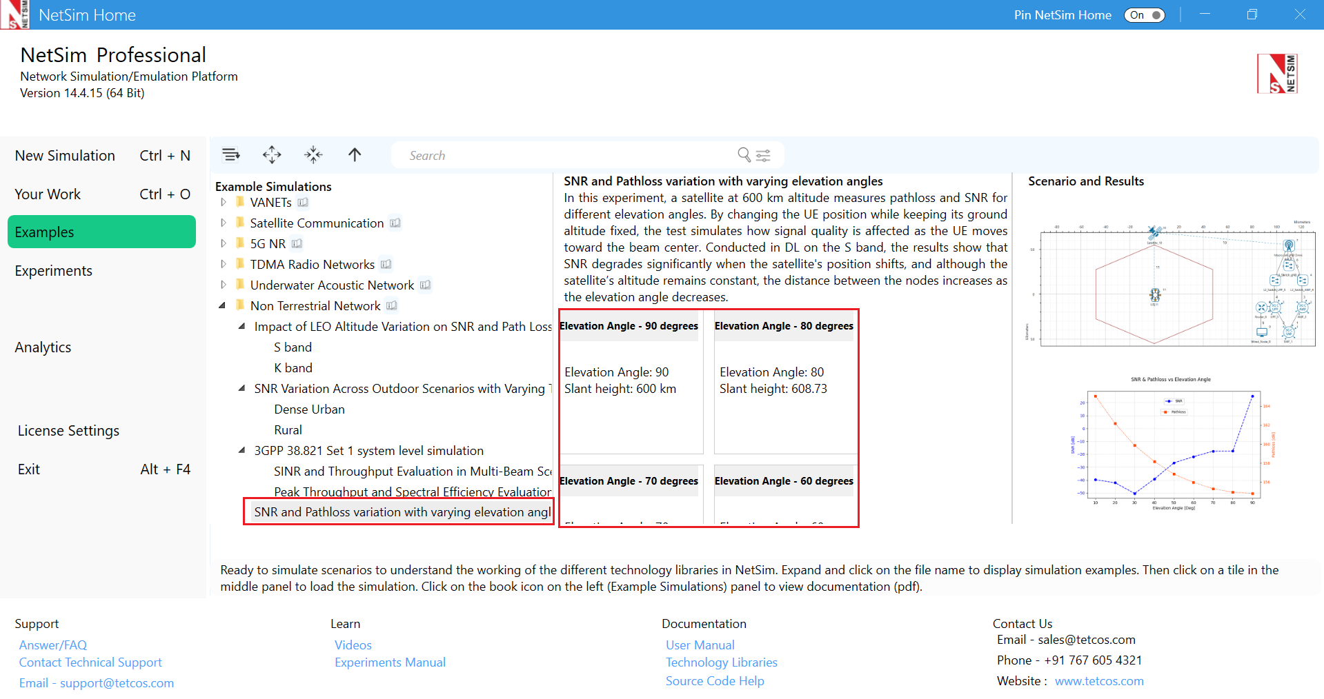
The following network diagram illustrates what the NetSim UI displays when you open the example configuration file.
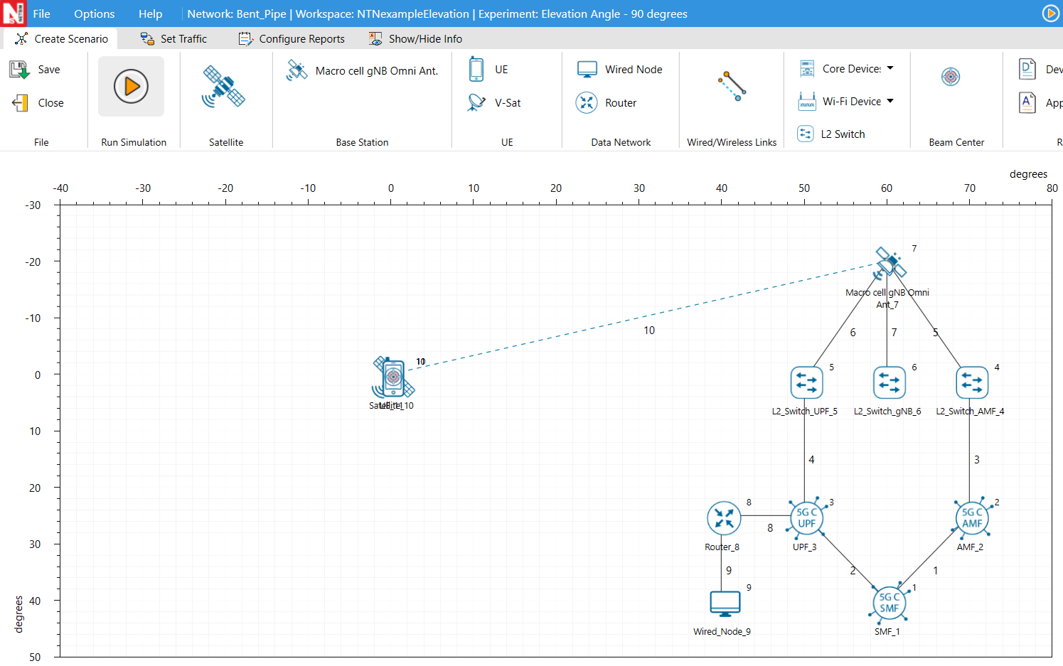
Settings in the example config file
| Elevation Angle | 90 | 80 | 70 | 60 | 50 | 40 | 30 | 20 | 10 |
|---|---|---|---|---|---|---|---|---|---|
| Slant height km | 600 | 608.29 | 634.78 | 682.83 | 760.90 | 882.24 | 1073.43 | 1393.22 | 1932.84 |
Results
Based on the UE position, the Elevation Angle and Slant Height (km) will change, these values can be observed from NTN UE Beam Association log.
3GPP 38.821 Set 1 system level simulation
Introduction
This simulation is based on the Set 1 Reference Scenario from 3GPP TR 38.821, which provides guidelines for evaluating the performance of Non-Terrestrial Networks (NTN) with Low Earth Orbit (LEO) satellites. In this setup, the satellite uses a transparent payload, meaning it acts as a relay, passing signals between the ground gateway and the User Equipment (UE).
Objective
The goal is to measure the distributions and percentiles of SINR and throughput across multiple spot beams, with each beam containing multiple UEs.
Part 1: Network Scenario
The following network diagram illustrates what the NetSim UI displays when you open the example configuration file.

Simulation Setup
To create this scenario, we have:
Set the Grid length to 450 \(\times\) 200
Dropped 19 beams in a hexagonal grid layout.
Randomly placed 10 UEs in each beam (total of 190).
Set the Band to S-band and Frequency reuse to FR1.
Selected LEO 600 from the orbit options to configure a Low Earth Orbit at 600 km altitude.
Simulation time is set to 30 seconds.
Parameter configuration
| Evaluation parameters | Values |
|---|---|
| Satellite \(\triangleright\) Interface_2 (Service link) properties | |
| Satellite Orbit | LEO 600 |
| Satellite altitude | 600 km |
| EIRP (dBW/MHz) | 34 |
| Antenna aperture (m) | 1 |
| Traffic | Full buffer DL |
| RU% | 100% |
| Elevation angle | Beam centres are at elevation angle \(90^{\circ}\). The UE’s elevation angle would depend on its location within the beam. |
| Antenna pattern | Bessel function per section 6.4.1 of TR 38.811. All UEs are not at the Nadir point and hence antenna gains need to be computed. |
| Additional loss(dB) | 0 |
| Clutter loss (dB) | 0 |
| UE density | 10 UEs per spot beam |
| Antenna temperature (k) | 290 |
| UE \(\triangleright\) Interface_1 (Service Link) properties | |
| UE Noise Figure (dB) | 7 |
| UE mobility | No mobility |
| gNB \(\triangleright\) Interface_4 (Feeder link) properties | |
| Band | S |
| CA Configuration | S Band n256 |
| Central Frequency (GHz) | 2.185 |
| Bandwidth (MHz) | 30 per beam |
| Downlink Scheduling Type | Round robin |
Application properties
Created a CBR application from Wired Node 9 to all UEs from the set traffic tab in the ribbon on top. Click on the created application, and in the right-side property panel, set the packet size to 1460B and Interarrival time to 584 \(\mu\)s, keeping the other application properties as default. This creates a generation rate of 20 Mbps ensuring full buffer at each UE.
| Application settings | ||
|---|---|---|
| Packet size(B) | 1460 | |
| Inter arrival time (\(\mu\)s) | 584 | |
| Generation rate (Mbps) | 20 | |
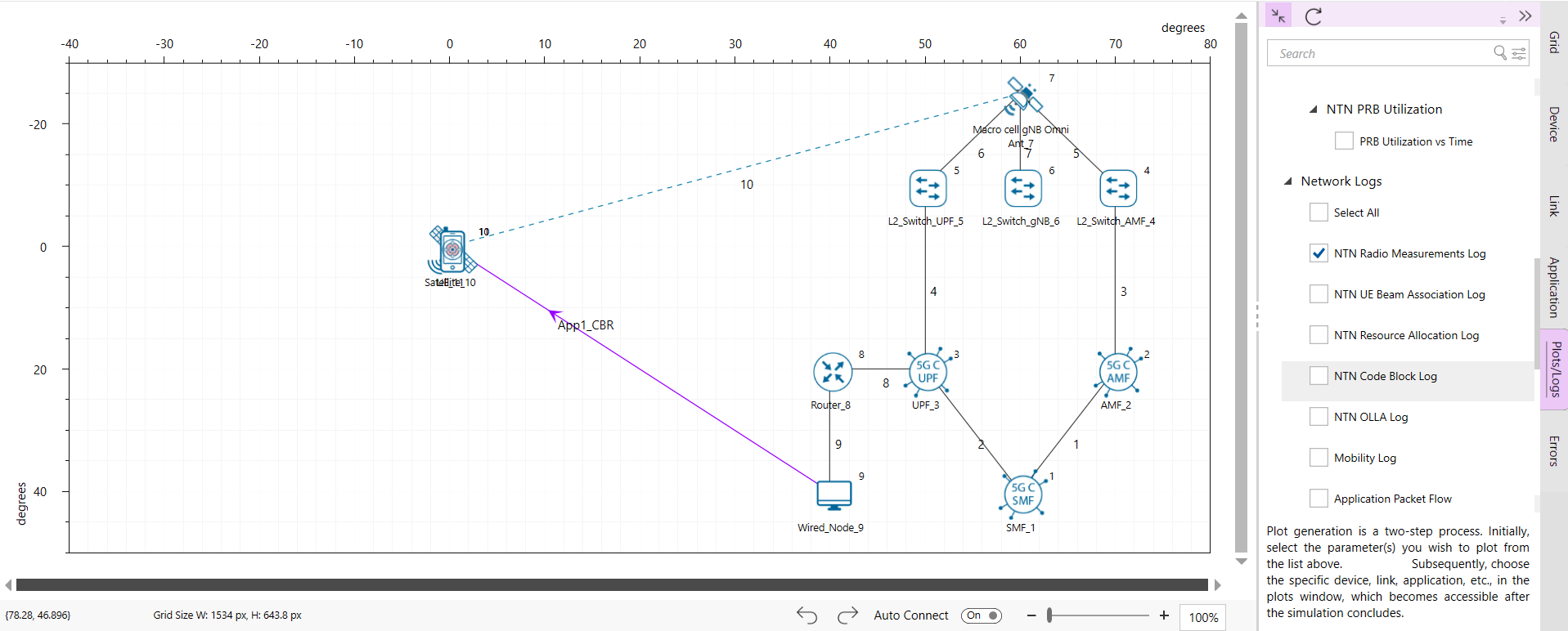
The NTN Radio measurement log, NTN Resource allocation log and Application packet flow log files must be enabled from the design window.
Log files can be enabled by clicking on the icon in Configure Reports \(\triangleright\) Plots \(\triangleright\) Network Logs option as shown below

Run simulation for 30s, after the simulation completes, go to results window click on logs options and open NTN Radio Measurement Log.csv, note down the SINR, and from the Application packet flow log note down the Throughput for each application.
Results and Discussion
The results of the simulation are shown using CDF plots for SINR, UE Throughput and Beam throughput.
To generate CDF of throughput plot, the Throughput column from the Application packet flow log file was considered, and the CDF of throughput was plotted.

| Throughput percentile metrics | |
|---|---|
| 5th percentile | 4.101 Mbps |
| 50th percentile | 7.473 Mbps |
| 95th percentile | 10.774 Mbps |
To generate CDF of SINR plot, the SINR column from the radio measurement log file was considered, and the CDF of SINR was plotted.

| SINR percentile metrics | |
|---|---|
| 5th percentile | 4.62 dB |
| 50th percentile | 10.47 dB |
| 95th percentile | 15.06 dB |
To generate CDF of per beam throughput plot, the throughput for each application was taken from the results window. The number of UEs associated with each beam was obtained from the resource allocation log file, and the CDF of throughput per beam was then plotted.

| Per-Beam Throughput percentile metrics | |
|---|---|
| 5th percentile | 61.79 Mbps |
| 50th percentile | 69.77 Mbps |
| 95th percentile | 78.97 Mbps |
The SINR CDF shows how the signal quality changes based on the user’s location within a beam. UEs near the beam center usually have better SINR, while edge UEs see lower values due to reduced antenna gain.
The throughput CDF shows how throughput is distributed among UEs. The scheduling is Round Robin scheduling and all UEs have full buffer traffic. UEs with higher SINR achieve slightly better throughput.
The per-beam throughput CDF shows how sum throughput varies across beams. Each beam has the same bandwidth and number of UEs, but performance depends on SINR which depends on UE location within the beam. Due to randomness in the UE positions we see a distribution in the per beam throughputs.
Satellite capacity
Satellite capacity = 1278.53 Mbps (Sum throughput of all 190 UEs)
Area Traffic capacity
Number of beams = 19
Beam radius, \(R\) = 55.13 km
Area per beam (A)= \(\frac{3\sqrt{3}}{2} R^{2}=\frac{3\sqrt{3}}{2}(55.13)^{2}=7887.1\) km\(^{2}\)
Total coverage area = \(7887.1 \text{ km}^{2}\times 19= 149854.9\) km\(^{2}\)
Area Traffic Capacity
\[\begin{equation} \frac{1278.53 \text{ Mbps}}{149854.9 \text{ km}^{2}}= 0.008531\times 1000 \text{ kbps/km}^{2}= 8.531 \text{ kbps/km}^{2} \end{equation}\]
Average Spectral efficiency
Channel Bandwidth = 30 MHz
Number of TRxPs = 19
\(\frac{\text{Aggregate Throughput(bps)}}{\text{Bandwidth}(Hz)\times \text{Number of TRxPs}}=\frac{1278.53\times 10^{6}}{30\cdot 10^{6}\times 19}=2.24\) bits/s/Hz/TRxP.
Part 2: Peak Throughput and Spectral Efficiency Evaluation
In this simulation scenario, 1 UE is placed at the nadir point, and the full system bandwidth of 30 MHz is allocated to that single user. The maximum number of Physical Resource Blocks (PRBs) supported by 30 MHz at numerology \(\mu = 0\) is 160 PRBs. A full buffer downlink traffic model is used, with a generation rate of 125 Mbps.
Network Scenario
The following network diagram illustrates what the NetSim UI displays when you open the example configuration file.
Simulation Setup
To create this scenario, we have:
Set the Grid length to 120 \(\times\) 40 km
Dropped a single beam in a hexagonal grid layout.
Placed the UE at the center of the beam footprint.
Set the Band to S-band and Frequency reuse to FR1.
Selected LEO 600 from the orbit options to configure a Low Earth Orbit at 600 km altitude.
Simulation time is set to 50 seconds.
Parameter configuration
| Evaluation parameters | Values |
|---|---|
| Satellite Orbit | LEO 600 |
| Satellite altitude | 600 km |
| Slant height | 600 km |
| EIRP (dBW/MHz) | 34 |
| Noise Figure (dB) | 7 |
| Antenna aperture (m) | 1 |
| Band | S |
| Frequency | 2 GHz (S Band) |
| Bandwidth (MHz) | 30 per beam |
| Downlink Scheduling Type | Round robin |
| Traffic | Full buffer DL |
| RU% | 100% |
| Elevation angle(\(^{\circ}\)) | 90 |
| Antenna pattern | Bessel function per section 6.4.1 of TR 38.811. |
| Pathloss (dB) | 154 |
| Additional loss (dB) | 0 |
| Clutter loss (dB) | 0 |
| UE density | 1 UE |
| UE mobility | No mobility |
| Antenna temperature (k) | 290 |
| UE TX power (dBm) | 23 |
| UE RX Antenna Gain (dB) | 0 |
Application Properties
Created a CBR application from Wired Node 9 to UE 11 from the set traffic tab in the ribbon on top. Click on the created application, and in the right-side property panel, set the packet size to 1460B and Interarrival time to 93.44 \(\mu\)s, keeping the other application properties as default. This creates a generation rate of 125 Mbps ensuring full buffer at each UE.
| Application settings | |
|---|---|
| Packet size(B) | 1460 |
| Inter arrival time (\(\mu\)s) | 93.44 |
| Generation rate (Mbps) | 125 |
Theoretical Spectral Efficiency Computation
As per Annex 1 of the ITU-2020-NTN framework, the theoretical peak spectral efficiency is given by:
\[\begin{equation} SE_{p} = \frac{v_{\text{Layers}}\cdot Q_{m}\cdot f\cdot R_{\max}\cdot\dfrac{N_{PRB}^{BW,\mu}\times 12}{T_{s}^{\mu}}\cdot(1-OH)}{BW} \end{equation}\]
The NTN code block log file must be enabled from the design window. MCS value can be observed from the code block log file.
Log file can be enabled by clicking on the icon in Configure Reports \(\triangleright\) Plots \(\triangleright\) Network Logs option as shown below
Where
Number of layer, \(\nu =1\)
Modulation order \(\left(Q_{m}\right)=6\)
Coding rate \(\left(R\right)=0.852\)
Numerology \(\left(\mu \right)=0\)
Overhead, \(OH = 0.14\)
Bandwidth \(=30\) MHz.
\(N_{PRB}^{BW,\mu}\)is the maximum Resource Block (RB) allocation in UE supported maximum bandwidth \(BW\) in a given band with numerology \(\mu\).
\(T_{s}^{\mu}\)is the average OFDM symbol duration in a subframe for numerology \(\mu\), i.e. \(T_{s}^{\mu}=\frac{10^{-3}}{14\times 2^{\mu}}\).
\(T_{s}^{\mu}=\frac{10^{-3}}{14\times 2^{\mu}} = \frac{0.001}{14}=0.00007143\)
\(\frac{N_{PRB}^{BW,\mu}\times 12}{T_{s}^{\mu}}(1-OH)=\frac{160\times 12\times (1-0.14)}{0.00007143}=23.11\times 10^{6}\)
\(SE_{p}=\frac{1\times 6\times 0.852\times 23.11\times 10^{6}}{30\times 10^{6}}=\frac{5.112\times 23.11}{30}=3.94\) b/s/Hz
Results and discussion
From the simulation results:
Achieved throughput = 105.65 Mbps
MCS Index = 21
Modulation = 64-QAM
Coding rate (R) = 0.852
Bandwidth \(=30\) MHz.
Observed Spectral Efficiency (SE) = \(\frac{\text{Achieved Throughput(bps)}}{\text{Bandwidth(Hz)}}= \frac{105.65 \times 10^{6} }{30\times 10^{6}}=3.52\) bits/sec/Hz
| Simulation Results | |
|---|---|
| Throughput (Mbps) | 105.65 |
| MCS | 21 |
| Spectral efficiency (bits/s/Hz) | 3.52 |
Thus, the theoretical peak spectral efficiency as per the ITU-2020-NTN Annex 1 formula is 3.94 bits/sec/Hz, while the observed spectral efficiency from the simulation is 3.52 bits/sec/Hz. This small gap reflects practical network conditions such as protocol overhead, scheduling inefficiencies, and real-time radio impairments.