Model Features

WLAN 802.11

NetSim implements the 802.11 MAC and the 802.11 PHY abstracted at a packet-level. We start with the 3 types of nodes supported in 802.11 Wi-Fi.

Wireless Nodes (Internetworks) or STAs. In Internetworks, APs and Wireless nodes (STAs) are associated based on the connecting wireless link
Wi-Fi Access Points (Internetworks) or APs. Every STA in the WLAN associates with exactly one AP. Each AP, along with its associated STAs, defines a cell. Each cell operates on a specific channel.
Standalone Wireless nodes (Mobile Adhoc networks).

The MAC Layer features:

RTS/CTS/DATA/ACK frame transmissions.
Packet queuing, aggregation, transmission, and retransmission.
802.11 EDCA.

The PHY layer implements:

RF propagation (documented separately).
Received power based on the propagation model.
Interference and signal to interference-plus-noise (SINR) calculation.
MCS (and in turn PHY Rate) setting based on RSS and rate adaptation algorithms.
BER calculation and packet error modelling.

WLAN standards supported in NetSim

802.11a, 802.11b, 802.11g, 802.11n, 802.11ac, 802.11ax, 802.11e (EDCA) and 802.11p are the WLAN standards available in NetSim. The operating frequencies and bandwidths are given in the Table‑1.

WLAN standard	Frequency (GHz)	Bandwidth (MHz)
802.11 a	5	20
802.11 b	2.4	20
802.11 g	2.4	20
802.11 p	5.9	5,10,20
802.11 n	2.4, 5	20, 40
802.11 ac	5	20, 40, 80, 160
802.11ax	2.4	20,40
802.11ax	5	20, 40, 80, 160

Table-1: WLAN standards supported in NetSim

802.11 p and WAVE are described in the VANET Technology library documentation.

The 2.4 GHz Channels

The following channel numbers are well-defined for the 2.4GHz standards:

Channel Number	Center Frequency (MHz)
1	2412
2	2417
3	2422
4	2427
5	2432
6	2437
7	2442
8	2447
9	2452
10	2457
11	2462
12	2467
13	2472
14	2484

Table-2: 2.4 GHz Wi-Fi Channels per IEEE Std 802.11g-2003, 802.11-2012 and 802.11-2024

Channels 1 through 14 are used in 802.11b, while channels 1 through 13 are used in 802.11g, 802.11n and 802.11ax.

The 5 GHz Channels

The following channel numbers are defined for 802.11a/n/ac/ax.

Channel Number	Center Frequency (MHz)
36	5180
40	5200
44	5220
48	5240
52	5260
56	5280
60	5300
64	5320
100	5500
104	5520
108	5540
112	5560
116	5580
120	5600
124	5620
128	5640
132	5660
136	5680
140	5700
144	5720
149	5745
153	5765
157	5785
161	5805
165	5825
169	5845
173	5865
177	5885

Table-3: 5GHz Wi-Fi Channels per IEEE Std 802.11a -1999, 802.11n -2009, 802.11ac -2013 , and 802.11ax-2021

The 5.9 GHz Channels

Channel Number	Center Frequency (MHz)
100	5500
104	5520
108	5540
112	5560
116	5580
120	5600
124	5620
128	5640
132	5660
136	5680
140	5700
171	5855
172	5860
173	5865
174	5870
175	5875
176	5880
177	5885
178	5890
179	5895
180	5900
181	5905
182	5910
183	5915
184	5920

Table-4: 5.9 GHz Wi-Fi Channels per IEEE Std 802.11p-2010

Channel Numbering

The standard method to denote 5 GHz channels is to use the 20 MHz center channel numbers, even when referring to wider channel widths (e.g., 40 MHz, 80 MHz, or 160 MHz). The following are the valid non-overlapping primary channels for 802.11n/ac/ax in NetSim:

20MHz: 36, 40, 44, 48, 52, 56, 60, 64, 100, 104, 108, 112, 116, 120, 124, 128, 132, 136, 140, 144, 149, 153, 157, 161, 165
40 MHz: 38, 46, 54, 62, 102, 110, 118, 126, 134, 142, 151, 159
80 MHz: 42, 58, 106, 122, 138, 155
160 MHz: 50, 114

WLAN PHY Rate in NetSim

WLAN Standard	Frequency (GHz)	Bandwidth (MHz)	MIMO streams	PHY rate (Mbps)
a	5	20	N/A	6, 9, 12, 18, 24, 36, 48, 54
b	2.4	20	N/A	1, 2, 5.5, 11
g	2.4	20	N/A	6, 9, 12, 18, 24, 36, 48, 54
n	2.4, 5	20	4	Up to 288
n	2.4, 5	40	4	Up to 600
ac	5	20	8	Up to 693.3
		40		Up to 1600.0
		80		Up to 3466.7
		160		Up to 6933.3
ax	2.4	20	8	Up to 1147
	2.4	40		Up to 2294
	5	20		Up to 1147
		40		Up to 2294
		80		Up to 4803
		160		Up to 9607

Table-5: WLAN PHY Rates in NetSim

SIFS, Slot Time, CW Min, and CW Max settings

Sub Std.	b (20MHz)
SIFS	10
Slot Time	20
CW Min	31
CW Max	1023

Table-6: DSSS PHY characteristics (IEEE-Std-802.11-2020 -Page no -2763 and 2764)

Sub Std.	a	g	p
Bandwidth	20MHz	20MHz	5MHz	10MHz	20MHz
SIFS	16	16	64	32	16
Slot Time	9	9	21	13	9
CW Min	15	15	15	15	15
CW Max	1023	1023	1023	1023	1023

Table-7: OFDM Physical Characteristics(IEEE-Std-802.11-2020 -Page no -2847)

Sub Std.	n
Frequency Band	2.4MHz	5
SIFS	10	16
Slot Time	20	9
CW Min	15	15
CW Max	1023	1023

Table-8: HT PHY characteristics (IEEE-Std-802.11-2020 -Page no -2952) and MIMO PHY characteristics (IEEE-Std-802.11n-2009 -Page no -335)

Sub Std.	ac (5GHz)
SIFS	16
Slot Time	9
CW Min	15
CW Max	1023

Table-9: Slot time in IEEE-Std-802.11-2020 -Page no -3094 and IEEE-Std-802.11ac-2013-Page no -297

Sub Std.	ax
Frequency Band	2.4MHz	5
SIFS	10	16
Slot Time	20	9
CW Min	15	15
CW Max	1023	1023

Table-10: The PHY characteristics (IEEE-Std-802.11-2024)

PHY Implementation

NetSim is a packet level simulator for simulating the performance of end-to-end applications over various packet transport technologies. NetSim can scale to simulating networks with 100s of end-systems, routers, switches, etc. It provides estimates of the statistics of application-level performance metrics such as throughput, delay, packet-loss, and statistics of network-level processes such as buffer occupancy, collision probabilities, etc.

To achieve scalable network simulation that can execute in reasonable time on desktop level computers, in all networking technologies the details of the physical layer techniques have been abstracted up to the point that bit-error probabilities can be obtained from which packet error probabilities are obtained.

NetSim does not implement any of the digital communication functionalities of the PHY layer. For PHY layer simulation, the modulation and coding scheme, along with the transmit power, path loss, noise, and interference, determine the bit rate and the bit error rate by using well-known formulas or tables for the particular PHY layer being used. Users would need to use a PHY Layer/RF/Link Level simulator for simulating various digital communication and link level functionalities. Typically, these simulators will simulate just one transmitter-receiver pair, rather than a network.

Generally, in NetSim, the PHY layer parameters available for the user to modify are Channel Bandwidth, Channel Centre Frequency, Transmit-power, Receiver-sensitivity, Antenna-gains, and the Modulation-and-Coding-Scheme. When simulating standard protocols, these parameters can only be chosen from a standard-defined set. NetSim also has standard models for radio pathloss; the parameters of these pathloss models can also be set.

PHY States

The PHY radio states implemented in NetSim 802.11 are RX ON IDLE, RX ON BUSY, TRX ON BUSY.

RX ON IDLE: This is the default radio state
RX ON BUSY: This state is set at receiver radio when the reception of data begins. Upon completion of reception it changes to RX ON IDLE
TRX ON BUSY: This state is set at the transmitter radio at the start of frame transmission. Upon completion of transmission, it changes to RX ON IDLE
A node in back off slots can be considered as equivalent to CCA busy. In NetSim, the radio state continues to be in RX ON IDLE
SLEEP state is not implemented since NetSim 802.11 does not currently implement power save mode.

802.11 implementation details

Packets arriving from the Network layer are queued in an access buffer, where they are sorted according to their priority per 802.11 EDCA. An event MAC OUT with Subevent CS (Carrier Sense – CSMA) is added to check if the medium is free

Figure-1: Packet transmission from the Network layer to the Mac Layer and how queued up in an access buffer.

During CS, if the medium is free, the NAV is checked. This occurs if the RTS/CTS mechanism is enabled, which can be done so by adjusting the RTS Threshold. If the Present Time > NAV, then an Event MAC OUT with Subevent DIFS End added at the time Present Time + DIFS time.

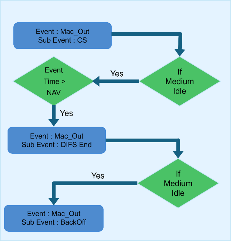
Figure-2: Event and Subevent in Mac layer

The medium is checked at the end of the DIFS time period. A random backoff is then calculated based on the Contention Window (CW). An Event MAC OUT with the Subevent BackOff is added at time Present Time + BackOff Time.

Once the backoff is successful, NetSim starts the transmission process by aggregating frames from the QoS Buffer and storing them in the Retransmit Buffer. If the A-MPDU size is greater than the RTS Threshold, the RTS/CTS mechanism is enabled, which is an optional feature.

Figure-3: Event and Subevent in Mac layer and Phy layer

NetSim sends the packet by calling the PHY OUT Event with Subevent AMPDU Frame. Note that the implementation of A-MPDU is in the form of a linked list.

Whenever a packet is transmitted, the medium is made busy and a Timer Event with Subevent Update Device Status is added at the transmission end time to set the medium again as idle.

Figure-4: Event and Subevent in Phy layer

Events PHY OUT Subevent AMPDU Subframe, Timer Event with the Subevent Update Device Status and Event PHY IN Subevent AMPDU Subframe are added in succession for each MPDU (Subframe of the aggregated frame). This is done for collision calculations. If two stations start transmission simultaneously, some of the Subframes may collide. Only those collided Subframes are retransmitted. The same logic is applied to errored packets. However, if the PHY header (the first packet) is errored or collided, the entire A-MPDU is resent.

At the receiver, the device de-aggregates the frame in the MAC Layer and generates a block ACK which is sent to the transmitter. If the receiver is an intermediate node, the de-aggregated frames are added to the access buffer of the receiver in addition to the packets which arrive from Network layer. If the receiver is the destination, then the received packets are sent to the Network layer. At the transmitter side, when the device receives the block acknowledgement, it retransmits only those packets which are errored. The rest of the packets are deleted from the retransmit buffer. This is done till all packets are transmitted successfully or a retransmit limit is reached after which next set of frames are aggregated to be sent.

802.11 ac/ax MAC and PHY Layer Implementation

Improvements in 802.11ac/ax compared to 802.11n

Feature	802.11n	802.11ac	802.11ax
Spatial Streams	Up to 4 streams	Up to 8 streams	Up to 8 streams
MIMO	Single User MIMO	Multi-User MIMO	Multi-User MIMO
Channel Bandwidth	20 and 40 MHz	20, 40, 80 and 160 MHz (optional)	20, 40, 80 and 160 MHz
Modulation	BPSK, QPSK, 16QAM, and 64QAM.	BPSK, QPSK, 16QAM, 64QAM and 256QAM (optional)	BPSK, QPSK, 16QAM, 64QAM, 256QAM and 1024 QAM
Max Aggregated Packet Size	65536 octets	1048576 octets	4,194,304 octets

Table-11: Feature Comparison between 802.11ac/ax to 802.11n

MAC layer improvements include only the increase in the number of aggregated frames from 1 to 64 .The MCS index for different modulation and coding rates are as follows:

MCS index	Modulation	Code Rate
0	BPSK	1/2
1	QPSK	1/2
2	QPSK	3/4
3	16QAM	1/2
4	16QAM	3/4
5	64QAM	2/3
6	64QAM	3/4
7	64QAM	5/6
8	256QAM	3/4
9	256QAM	5/6
10 (11ax only)	1024 QAM	3/4
11 (11ax only)	1024 QAM	5/6

Table-12: Different Modulation schemes and Code Rates

Receiver sensitivity for different modulation schemes in 802.11ac/ax (for a 20MHz Channel bandwidth) are as follows.

MCS Index	Receiver Sensitivity (in dBm)
0	-82
1	-79
2	-77
3	-74
4	-70
5	-66
6	-65
7	-64
8	-59
9	-57
10	-54
11	-52

Table-13: MCS index vs. Receiver Sensitivity (Rx-sensitivity)

The Rx-sensitivity is then set per the above table in conjunction with Max Packet Error Rate (PER) as defined in the standard.

If users wish to apply just the Rx-sensitivity (also termed as rate dependent input level), then the calculate_rxpower_by_per() function call in the function

fn_NetSim_IEEE802_11_HTPhy_UpdateParameter() in the file IEEE802_11_HT_PHY.c(equivalent functions in IEEE802_11_HEPhy.c) can be commented.

Number of subcarriers for different channel bandwidths

PHY Standard	Subcarriers	Capacity relative to 20MHz in 802.11ac
802.11n/802.11ac 20MHz	Total 64, 52 Data, 4 pilot	x1.0
802.11n/802.11ac 40MHz	Total 128, 108 Data, 6 pilot	x2.1
802.11ac 80MHz	Total 256, 234 Data, 8 pilot	x4.5
802.11ac 160MHz	Total 512, 468 Data, 16 pilot	x9.0

Table-14: Number of subcarriers for different channel bandwidths

PHY Standard	Subcarriers	Capacity relative to 20MHz in 802.11ac
20 MHz	Total 256, 234 Data, 8 pilot	x1.65
40 MHz	Total 512, 468 Data, 16 pilot	x3.3
80 MHz	Total 1024, 980 Data, 16 pilot	x6.92
160 MHz	Total 2048, 1960 Data, 32 pilot	x13.85

Table-15: Number of subcarriers for different channel bandwidths (11ax HE SU OFDM)

With the knowledge of MCS index and bandwidth of the channel data rate is set in the following manner

Get the number of subcarriers that are usable (data) for the given bandwidth of the medium.
Get the Number of Bits per Subcarrier (NBPSC) from selected MCS
Number of Coded Bits Per Symbol (NCBPS) = NBPSC*Number of Subcarriers
Number of Data Bits Per Symbol (NDBPS) = NCBPS*Coding Rate
Physical level Data Rate = NDBPS/Symbol Time (For 802.11n/ac, the total OFDM symbol duration is 3.6 microseconds with a 0.4 µs (short) Guard Interval and 4 microseconds with a 0.8 µs (long) Guard Interval. In 802.11ax, the total OFDM symbol durations are 13.6 µs, 14.4 µs, and 16 µs corresponding to Guard Intervals of 0.8 µs, 1.6 µs, and 3.2 µs, respectively.)

MAC Aggregation in NetSim

NetSim supports A-MPDU aggregation and does not support A-MSDU aggregation. MAC Aggregation is independent of MCS (PHY Rate) or BER. It is the PHY Rate that adapts to BER via Rate Adaptation algorithms.

In the aggregation scheme shown in Figure 3 5, several MPDU’s (MAC Protocol Data Units) are aggregated into a single A-MPDU (Aggregated MPDU). The A-MPDUs are created before transfer to the PHY. The MAC does not wait for MPDUs to aggregate. It aggregates the frames already queued to form an A-MPDU. The maximum size of an A-MPDU is 46,92,480 bytes.

Figure-5: Aggregation scheme

In 802.11n, a single block acknowledgement is sent for the entire A-MPDU. The block ack acknowledges each packet that is received. It consists of a bitmap (compressed bitmap) of 64bits or 8 bytes. This bitmap can acknowledge up to 64 packets, 1 bit for each packet.

The value of a bitmap field is 1, if respective packet is received without error else it is 0. Only the error packets are present until a retry limit is reached. The number of packets in an A-MPDU is restricted to 64 since the size of block ack bitmap is 64bits.

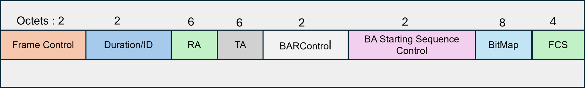
Figure-6: Block Ack Control Packet

NetSim uses the parameter Number of frames to aggregate, while the standard uses the parameter A-MPDU Length Exponent. Per standard the A-MPDU length is defined by two parameters: Max AMPDU length exponent and BLOCK ACK Bitmap. The AMPDU length in bytes is \(2^{(13 + MaximumAMPDULengthExponent)} - 1\ \).
Since NetSim doesn't model A-MSDU, a design decision was made to model A-MPDU based on Block ACK bitmap size (to indicate the received status of up to 64 frames) and therefore the parameter - Number of Frames to Aggregate - in the GUI
When EDCA is enabled, packet aggregation is done separately for each QoS class
NetSim ignores the padding bytes added to the MPDU
The MAC aggregates packets destined for the same receiver, regardless of the end destination. The receiver is to be understood as the next hop in a wireless transmission.
The RTS threshold is compared against the total A-MPDU size.
Aggregation functionality may not execute correctly if:

\[NumberOfFramesToAggregate \times PacketSize\ (B) > 46,92,480\ (B)\]

Signal to interference and noise ratio (SINR)

At each receiver, when the first packet is transmitted and every time the transmitter or receiver moves, NetSim calculates the received signal level from the transmitter. The received signal level would be equal to transmit power less propagation losses. Next, NetSim calculates the interference received (at the same receiver), from all the interfering transmissions. Only co-channel interference is accounted for, and adjacent channel interference is not calculated. Finally, NetSim takes the ratio of the signal level, to the sum of the total interference from other transmissions plus the thermal noise. This ratio is SINR.

Once the SINR is calculated the BER is obtained from the SINR-BER tables for the applicable modulation scheme. This BER is then converted to Packet-Error-Rate. Packet error (Yes/No) is determined by drawing a random number in (0, 1) and comparing against PER.

The same is explained diagrammatically below.

Figure-7: Radio Tx-Rx for one transmission.

* Propagation model covers path loss, fading and shadowing. The models are documented in a separate document named Propagation-Models.pdf.

** Interference noise due to other transmissions within the network

Error Model

BER by Table: Packet Error Probability (PEP) is derived from SINR-MCS (Signal-to-Interference-plus-Noise Ratio - Modulation and Coding Scheme) lookup tables, as referenced in the Cisco document available at https://community.cisco.com/legacyfs/online/attachments/discussion/revolution-wi-fi-mcs-to-snr-single-page.pdf. They map specific SINR values to Bit Error Rates (BER), which are then used to calculate the probability of packet errors. These tables are implemented in the SINR-BER.c file, which is part of the medium project. Users can edit these table entries to tailor the simulation to specific needs or scenarios.
BER by formula: The Bit Error Rate (BER) is derived from SINR-BER formulas outlined in section 6 of the NetSim manual propagation-model.pdf. The packet error probability (PEP) is calculated from the BER by considering the packet length.

Transmit Power

The user can set a fixed transmit power via the GUI. Transmit power is a local variable, allowing each STA and AP to have unique transmit power settings. The transmit power can be dynamically varied by modifying the underlying 802.11 source C code.

Carrier Sense

Transmit power less propagation losses is the received power. The propagation loss is the sum (in dB scale) of pathloss, shadowing loss and fading loss. Various propagation models are available and are detailed in the Propagation model manual. Pathloss, Fading, and Shadowing can be turned on/off in GUI.

If \(ReceiverSensitivity(Lowest\ MCS) \geq \ Receiver - Power \geq ED - Threshold,\) the medium is set to busy. Note that CSMA/CA algorithm operates according to the medium state (busy/idle).

If \(Received - Power > Reciver - Sensitivity\ (LowestMCS)\) then MCS is set depending on the received power and signal is decoded. Packet errors are decided by looking up the SINR-BER table for the given MCS.

The variables can also be modified dynamically by changing the underlying 802.11 source C code

Transmission Range, Carrier Sense Range, and Interference Range

Transmission Range: The transmission range is the range within which the receiver of a signal can decode the source’s transmission correctly (when no other transmitting node’s signal interferes). This is typically smaller than the carrier-sensing range of the transmitter.
Carrier Sense Range: The carrier-sense range is the range within which the transmitter’s signal exceeds the Carrier Sense Threshold of the receiver (or another transmitter). The receiver (or another transmitter) detects the medium to be busy and does not transmit at this time.
Interference Range: The interference range (defined by the receiver) is the range within which any signal transmitted by other sources interfere with the transmission of the intended source, thereby causing a loss (marked as a collision in NetSim) at the receiver.

These three ranges are affected by the power of the transmitter. The greater the transmission power, the further a node can receive the transmission, and also the more nodes whose communication with other nodes will be affected by this transmission. The transmission range is also affected by the MCS used by the transmitter. The higher the MCS the shorter the range, and vice versa

Carrier Sense (CS) Threshold

In NetSim (from v13.2 onwards) the Carrier sense (CS) threshold is set equal to Control rate receive sensitivity.

\[CSThreshold = RecieverSensitivity(ControlRate)\]

Users can modify the CS Threshold using the variable CSRANGEDIFF which is set to 0 dB in code by default. This implies a 0 dB differential between the lowest MCS (Control rate) Receive sensitivity (which determines DecodeRange) and CS Threshold (which determines CarrierSenseRange). The value of CSRANGEDIFF can be modified by the user in NetSim Standard or Pro versions, which ship with source code. We believe the term EDThreshold used in literature is the same as CSThreshold.

If the interference signal power (sum of the Received-power from all other transmitters), measured at the transmitter, is greater than ED-Threshold, then the transmitter assumes the medium is busy. Carrier is sensed by the transmitter; all CS activity occurs at the transmitter, and not at the receiver

Transmitter’s choice of MCS

If the Rate Adaptation algorithm is turned off, then the transmitter chooses MCS by comparing the RSS (calculated per the equation below) against the Receiver-Sensitivity for different MCS (per the tables in the standards). The highest possible MCS is chosen. This means the MCS is not fixed but adapts to the received signal strength, even with rate adaption turned off in the MAC layer.

NetSim exploits the AP-STA and the STA-AP channel reciprocity. Therefore, pathloss plus shadow loss is identical in both directions.

\[RSSI = TxPower - Pathloss - ShadowLoss\]

Note that when computing BER (from SINR) fading loss is added to this RSSI value. Thus, fading loss is not accounted for when choosing MCS, but is accounted for when computing BER.

NetSim has rate adaptation algorithms which take care of selecting the right MCS for a given SINR. In the simplest algorithm for every 20 successful transmissions the rate (MCS) goes up 1 step, and for every 3 continuous failures, the rate goes down one step.

Hidden Node Behavior

Consider N1 and N3 transmitting to N2 where N1 and N3 are beyond Carrier sense (CS) range. N1 is said to be hidden from N3 and vice versa.

When N1 and N3 transmit, there are likely to be collisions at N2. However, collisions do not occur all the time. The CSMA/CA algorithm exponentially increases the backoff and hence after a few collisions it is possible that one of the nodes gets a low back-off number while the other draws a very high back-off number. Thus, the node with low back-off can complete transmissions (of one and even more than one packet) while the other node (with the large backoff) is still in backoff.

When N1 transmits to N2, N3 can’t hear the transmission since N3 is beyond CS. Therefore, N3 can attempt if its backoff counts down to 0. However, when N2 sends back the WLAN-ACK, N3 will hear it since N3 is within range of N2. Therefore, in NetSim, N3 will sense the medium as busy and freeze its back off when N2 is sending the WLAN ACK to N1.

In case of N2 to N1/N3 transmissions, then the reverse is true for the MAC-ACK from the nodes. When N2 sends a packet to N1 (or N3) it is within range of N3 (or N1), however, when N1 (or N3) sends back the MAC ACK there is a chance of collision with a data packet of N3 (or N1).

IEEE 802.11 e QoS and EDCA

Quality of Service (QoS) provides you with the ability to specify parameters on multiple queues for increased throughput and better performance of differentiated wireless traffic like Voice-over-IP (VoIP), other types of audio, video, and streaming media, as well as traditional IP data over the Access Point.

QoS was introduced in 802.11e and is achieved using enhanced distributed channel access functions (EDCAFs). EDCA provides differentiated priorities to transmitted traffic, using four different access categories (ACs). With EDCA, high-priority traffic has a higher chance of being sent than low-priority traffic: a station with high priority traffic waits a little less before it sends its packet, on average, than a station with low priority traffic. This differentiation is achieved through varying the channel contention parameters i.e., the amount of time a station would sense the channel to be idle, and the length of the contention window for a backoff.

In addition, EDCA provides contention-free access to the channel for a period called a Transmit Opportunity (TXOP). A TXOP is a bounded time interval during which a station can send as many frames as possible (as long as the duration of the transmissions does not extend beyond the maximum duration of the TXOP). If a frame is too large to be transmitted in a single TXOP, it should be fragmented into smaller frames. The use of TXOPs reduces the problem of low rate stations gaining an inordinate amount of channel time in the legacy 802.11 DCF MAC. A TXOP time interval of 0 means it is limited to a single MPDU.

Figure-8: Enhanced Distributed Channel Access (EDCA) in 802.11

NetSim categorizes application packets based on QoS class set in application properties as follows

VO: UGS and RTPS
VI: NRTPS and ERTPS
BE: BE and all control packets such as TCP ACKs
BK: Everything else

Default EDCA Parameters

The following tables show the default EDCA parameters. This default parameter set is per page 899, IEEE Std 802.11-2016

Access Category	CW min	CW max	AIFSN	Max TXOP (\(\mathbf{\mu s}\))
Background (AC-BK)	31	1023	7	3264
Best Effort (AC-BE)	31	1023	3	3264
Video (AC-VI)	15	31	2	6016
Voice (AC-VO)	7	15	2	3264

Table-16: Default EDCA access parameters for 802.11 b for both AP and STA

Access Category	CW min	CW max	AIFS N	Max TXOP (\(\mathbf{\mu s}\))
Background (AC-BK)	15	1023	7	2528
Best Effort (AC-BE)	15	1023	3	2528
Video (AC-VI)	7	15	2	4096
Voice (AC-VO)	3	7	2	2080

Table-17: Default EDCA access parameters for 802.11 a / g / n / ac / ax for both AP and STA

Access Category	CWmin	CWmax	AIFSN
Background (AC-BK)	15	1023	9
Best Effort (AC-BE)	15	1023	6
Video (AC-VI)	7	15	3
Voice (AC-VO)	3	7	2

Table-18: Default EDCA access parameters for 802.11 p (dot11OCBActivated is true)

The EDCA parameters can be configured by changing the Physical type parameter according to the different standard, IEEE802.11b (Medium Access Protocol 🡪 DSSS), IEEE802.11n (Medium Access Protocol 🡪 HT), IEEE802.11ac (Medium Access Protocol 🡪 VHT), IEEE 802.11ax (Medium Access Protocol HE), IEEE802.11a and g (Medium Access Protocol 🡪 OFDMA and OCBA 🡪FALSE), IEEE802.11p (Medium Access Protocol 🡪 OFDMA and OCBA 🡪TRUE).

Rate Adaptation

In NetSim (with default code), rate adaptation works as follows:

FALSE: This is similar to Receiver Based Auto Rate (RBAR) algorithm. In this, the PHY rate gets set based on the target PEP (packet error probability) for a given packet size, as given in the standard. The adaptation is termed as “FALSE” since the rate is pre-determined as per standard and there is no subsequent “adaptation”.

802.11 n/ac/ax: Target PEP = 0.1, Packet Size: 4096 B

802.11 b: Target PEP = 0.08, Packet Size: 1024B

802.11 a/g/p: Target PEP:0.1, Packet size 1000B

GENERIC: This is similar to the Auto Rate FallBack (ARF) algorithm. In this algorithm:

Rate goes up one step for 20 consecutive packet successes

Rate goes down one step for 3 consecutive packet failures

MINSTREL: Per the minstrel rate adaptation algorithm implemented in Linux

Model Limitations

Mobility of Wireless nodes is not available in infrastructure mode (when connected via an Access Point) and is only available in Adhoc mode. Hence mobility for wireless nodes can only be set when running MANET simulations.
Authentication and encryption are not supported
While different APs can operate in different channels, all the Wireless nodes connected to one AP operate in the same channel.
No beacon generation, probing or association
RTS, CTS and ACK are always transmitted at the base rate (lowest MCS)
Roaming whereby a STA leaves serving AP to associate with target AP (usually based on RSSI/SNR)

Wi-Fi GUI Parameters

The WLAN parameters can be accessed by clicking on an Access Point or Wireless Node, then going to the right-hand side panel and expand Interface (Wireless) Properties -> Datalink and Physical Layers

Access Point and Wireless Node Properties
Interface Wireless – Datalink Layer
Parameter	Scope	Range	Description
Rate Adaptation	Cell	False	There is no rate adaptation, and the rate depends on the MCS selection option chosen in the PHY layer.
		Minstrel	Operates similar to the rate adaptation algorithm implemented in Linux
		Generic	In this algorithm (i) Rate goes up one step for 20 consecutive packet successes, and (ii) Rate goes down one step after 3 consecutive packet failures.
Short Retry Limit	Local	1 to 255	Determines the maximum number of transmission attempts of a frame. The length of MPDU is less than/ equal to Dot11 RTS Threshold value, made before a failure condition is indicated.
Long Retry Limit	Local	1 to 255	Determines the maximum number of transmission attempts of a frame. The length of MPDU is greater than Dot11 RTS Threshold value, made before a failure condition is indicated.
Dot11 RTS Threshold	Local	0 to 4692480	The size of packets (or A-MPDU if applicable) above which RTS/CTS (Request to Send / Clear to Send) mechanism gets triggered.
MAC Address	Fixed	Auto Generated	The MAC address is a unique value associated with a network adapter. This is also known as hardware address or physical address. This is a 12-digit hexadecimal number (48 bits in length).
Buffer Size	Local	1 to 100	Buffer is the memory in a device which holds data packets temporarily. If incoming rate is higher than the outgoing rate, incoming packets are stored in the buffer. NetSim models the buffer as an egress buffer. Unit is MB.
Medium Access Protocol	Local	DCF	DCF is the process by which CSMA/CA is applied to Wi-Fi networks. DCF defines four components to ensure devices share the medium equally: Physical Carrier Sense, Virtual Carrier Sense, Random Back-off timers, and Interframe Spaces (IFS). DCF is used in non-QoS WLANs.
Medium Access Protocol	Local	EDCAF	QoS was introduced in 802.11e and is achieved using enhanced distributed channel access functions (EDCAFs). EDCA provides differentiated priorities to transmitted traffic, using four different access categories (ACs). With EDCA, high-priority traffic has a higher chance of being sent than low-priority traffic: a station with high priority traffic waits a little less before it sends its packet, on average, than a station with low priority traffic.
Physical Type	Global	DSSS	Direct Sequence Spread Spectrum. The physical type parameter is set to DSSS if the standard selected is IEEE802.11b.
		OFDM	Orthogonal Frequency Division Multiplexing is utilized as a digital multi-carrier modulation method. The physical type parameter is set to OFDM if the standard selected is IEEE802.11a, g and p.
		HT	Operates in frequency bands 2.4GHz or 5GHz band. The physical type parameter is set to HT if the standard selected is IEEE802.11n.
		VHT	The physical type parameter is set to VHT if the standard selected is IEEE802.11ac.
		HE	Operates in frequency bands 2.4 GHz or 5 GHz band. The physical type parameter is set to HE if the standard selected is IEEE802.11ax.
OCBA Activated	Local	True or False	This parameter determines the type of standard to be chosen for the OFDM physical type. The standard is set to IEEE802.11p if OCBA is True. The standard is set to IEEE802.11a and g if OCBA is False.
BSS Type	Fixed	Auto Generated	The BSS type is fixed to Infrastructure mode. The wireless device can communicate - with each other or with a wired network - through an Access Point.
CW min (Slots)	Local	0 to 255	Specifies the initial Contention Window (CW) used by an Access Point (or STA) for a particular AC for generating a random number for the back-off.
CW max (Slots)	Local	0 to 65535	At each collision the CW is doubled. \(CW_{Max}\) specifies the final maximum CW values used by an Access Point (or STA) for a particular AC for generating a random number for the back-off.
AIFSN (Slot)	Local	2 to 15	Specifies the number of slots after a SIFS duration.
Max TXOP	Local	0 to 65535	Specifies the maximum number of microseconds of an EDCA TXOP for a given AC. Unit is microseconds.
MSDU Lifetime (TU)	Local	0 to 500	Specifies the maximum duration an MSDU would be retained by the MAC before it is discarded, for a given AC. MSDU Lifetime is specified in TU.
Interface Wireless- Physical Layer
Protocol	Fixed	IEEE 802.11	Defines the MAC and PHY specifications like IEEE802.11a/b/g/n/ac/ax/p for wireless connectivity for fixed, portable and moving stations within a local area.
Connection Medium	Fixed	Auto Generated	Defines how the devices are connected or linked to each other.
Standard	Cell	IEEE 802.11 a/b/g/n/ac/ax/p	Refers to a family of specifications developed by IEEE for WLAN technology. The IEEE standards supported in NetSim are IEEE 802.11 a, b, g, n, ac, ax and p. 802.11a provides up to 54 Mbps in 5 GHz band. 802.11b provides 11 Mbps in the 2.4 GHz bands. 802.11 g provides 54 Mbps transmission over short distances in the 2.4 GHz band. 802.11 n adds up MIMO. 802.11 ac supports wider channels and includes beamforming capabilities. 802.11 p provides support to Intelligent Transportation Systems.
Transmission Type	Fixed	DSSS	The transmission type parameter is DSSS if the standard selected is IEEE802.11b.
		OFDM	The transmission type parameter is OFDM if the standard selected is IEEE802.11a, g and p.
		HT	The transmission type parameter is HT if the standard selected is IEEE802.11n.
		VHT	The transmission type parameter is VHT if the standard selected is IEEE802.11ac.
Number of Frames to Aggregate	Cell	1 to 1024 (11ax) 1 to 64 (11ac) 1 to 64 (11n)	Number of frames aggregated to form an A-MPDU. This is fixed and cannot be dynamically varied (except by modifying the code). See 3.1.12 for more information.
Transmit Power	Local	0 to 1000	Transmitted signal power. Note that the transmit power is not split among the antennas. This value is applied to each antenna in a multi-antenna transmitter. Unit is mW.
Antenna Gain	Local	0 to 1000	A relative measure of an antenna’s ability to direct or concentrate radio frequency energy in a particular direction or pattern. The measurement is typically measured in dBi (Decibels relative to an isotropic radiator).
Antenna Height	Local	0 to 100m	It is used in the pathloss calculation in the following models: Cost231 Hata Urban, Cost231 Hata SubUrban, Hata Urban, Hata SubUrban and Two Ray. This parameter has no effect when using any of the other pathloss models. Default:0.0 m.
SIFS	Fixed	Auto Generated	The time interval required by a wireless device in between receiving a frame and responding to the frame. Unit is microseconds.
Frequency Band	Cell	2.4, 5 (Depends on the standard chosen)	Range of frequencies at which the device operates. The frequency band depends on the standard selected. Unit is GHz.
Bandwidth	Cell	20, 40, 60, 80, 160 (Depends on the standard chosen)	The bandwidth depends on the standard and the frequency band selected. Unit is MHz
CCA Mode	Fixed	Auto Generated	A mechanism to determine whether a medium is idle or not. It includes Carrier sensing and energy detection.
Slot Time	Fixed	Auto Generated	Time is quantized as slots in Wi-Fi. Unit is microseconds.
Standard Channel	Local	Depends on the standard chosen	The channel options defined in the standards. The options would also depend on the frequency band if the standard supports multiple bands.
CW Min	Fixed	Auto Generated	The minimum size of the Contention Window in units of slot time. The CW min is used by the MAC to calculate the back off time for channel access during a carrier sense.
CW Max	Fixed	Auto Generated	The maximum size of the Contention Window in units of slot time. The CW is doubled progressively when collisions occur.
Transmitting Antennas	Local	1 to 8	The number of transmit antennas. Note that power is not split among the transmit antennas but is assigned to each antenna. (The pair of Tx and Rx antenna present only for 802.11ac and 802.11n)
Receiving Antennas	Local	1 to 8	The number of receive antennas
Guard Interval	Local	400 and 800 800, 1600 and 3200ns (11ax)	Guard Interval is intended to avoid signal loss from multipath effect. Unit is nanoseconds.
MCS Selection	Local	Auto Rate Fallback, Fixed	MCS selection in Wi-Fi impacts data rates and efficiency. Auto Rate Fallback adapts the MCS based on signal quality (RSSI) per the RSSI-MCS tables in the 802.11 standards. Fixed MCS locks the MCS. Default Value: Auto Rate
Data MCS	Local	802.11b: 0-3 802.11a/g/p: 0-7 802.11n: 0-7 802.11ac: 0-9 (MCS 9 not available for 20MHz in VHT) 802.11ax: 0-11	Allows selection of the MCS value for different Wi-Fi standards. Determines the modulation and coding scheme. Default Value: 0.
Data PHY Rate (Mbps)	Local	Determined by selected Data MCS and Wi-Fi standard	Shows the physical layer data rate based on the chosen modulation and coding scheme. (MCS)
Error Model	Local	SINR-BER-By-Table, SINR-BER-By-Formula	Specifies how the Bit Error Rate (BER) is calculated: BER is determined based on predefined tables mapping SINR to BER. BER is calculated using mathematical formulas that account for the modulation and coding schemes used, based on the SINR value.

Table-19: Internetworks Config Properties

IEEE 802.11 Results

IEEE 802.11 performance metrics will be displayed in the results dashboard if the network scenario simulated consisted of at least one device with WLAN protocol enabled.

Parameter	Description
Device Id	It represents the Id of the wireless device which supports 802.11 (WLAN)
Interface Id	It represents the interface Id’s of the wireless nodes
Frame Sent	It is the Number of frames sent by Access Point
Frame Received	It is the number of frames received by a wireless node
RTS Sent	It is the number of Request to send (RTS) packets sent by a Wireless Node. RTS/CTS frames are sent prior to transmission when the packet size exceeds the RTS threshold. The access point receives the RTS and responds with a CTS frame. The station must receive a CTS frame before sending the data frame. The CTS also contains a time value that alerts other stations to hold off from accessing the medium while the station initiating the RTS transmits its data.
RTS Received	It is the number of RTS packets received by an Access Points
CTS Sent	It is the number of Clear to send (CTS) packets sent by an Access Points
CTS Received	It is the number of CTS packets received by Wireless Nodes
Successful BackOff	It is the number of successful backoffs running at a wireless node. In the IEEE 802.11 Wireless Local Area Networks (WLANs), network nodes experiencing collisions on the shared channel need to BackOff for a random period of time, which is uniformly selected from the Contention Window (CW). BackOff is a timer which is decreased as long as the medium is sensed to be idle for a DIFS, and frozen when a transmission is detected on the medium, and resumed when the channel is detected as idle again for a DIFS interval
Failed BackOff	It is the number of failed backoffs at wireless node

Table-20: Description of IEEE 802.11 Metrics

Radio measurements log file

NetSim IEEE 802.11 Radio measurements csv log file records pathloss, shadowing loss, fading loss, transmitted power, received power, SNR, Interference Power, SINR, BER, NSS, MCS. This log can be enabled by clicking on configure reports in top ribbon > Plots > Select IEEE 802.11 Radio Measurements log under Network Logs as shown below

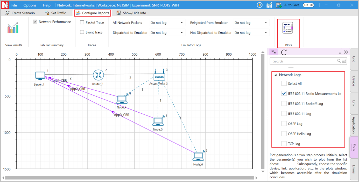
Figure-9: Enabling IEEE 802.11 Radio Measurement log.

The IEEE 802.11 Radio Measurement log.csv file will contain the following information:

Time in Milliseconds
Transmitter Name
Receiver Name
Distance between the Transmitter and the Receiver in meters
Packet ID
Packet Type
Control Packet Type
Transmitter Power in dBm
Total Loss in dB
Pathloss in dB
Shadowing Loss in dB
Fading Loss in dB
Received Power in dBm
Interference in dBm
Tx Antenna Gain(dB)
Rx Antenna Gain(dB)
SNR in dB
SINR in dB
BER
NSS
MCS

The log file can be accessed from the Simulations Results Window under the Logs option as shown below

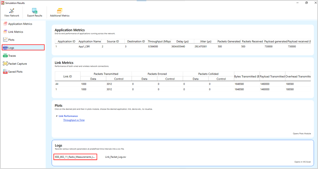
Figure-10: IEEE 802.11 Radio Measurement log.csv file highlighted in the Results window.

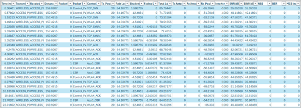
Figure-11: IEEE 802.11 Radio Measurement log.csv file.

Implementation details and Assumptions:

The log is written during each packet received at the physical layer (PHY_IN). Hence the number of entries will be based on the number of packets received, by all nodes or specific nodes based on values present in the DEVICE ID LIST array.
The MCS column displays the MCS index from the Phy parameters table in case of IEEE 802.11 n ac and ax. However, it displays the index value from the Phy parameters table as nIndex-1 in case of DSSS based standards such as b and OFDM based standards such as a, g and p.
The NSS value is currently set to the minimum of transmit and receive antenna counts in the same device. For example, if Transmitting Antennas is set to 2 and receiving Antennas is set to 8 then NSS is set to 2.

NetSim plots

NetSim also provides Wi-Fi radio measurement plots. Enabling the plots is explained in the section "Enable protocol specific logs and plots". Here is the plot showing the SNR vs. time for a scenario involving three wireless nodes connected to a single AP, with the wireless nodes placed at different distances

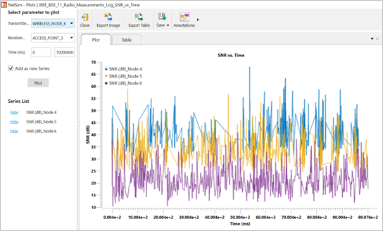
Figure-12: Plot of SNR vs Time for Internetworks Wi-Fi scenario.

IEEE 802.11 Backoff Log

NetSim 802.11 Backoff log file records details such as the Device name, Time stamp, Packet ID, BackoffTime, contention Window size and Retry Limit. This log can be used to understand the medium access mechanism in IEEE 802.11 Protocols.

This log file can be enabled in NetSim GUI by clicking on Plots tab > Network Logs > IEEE 802.11 Backoff Log on the right panel as shown below.

Figure-13: Enabling IEEE 802.11 Backoff log.

The IEEE802 11 Backoff Log.csv file will contain the following information:

Device Name
Timestamp
Packet ID
BackOffTime
Contention Window Size
Retry Limit

The log file can be accessed from the Simulations Results Window under the Logs option in the left pane.

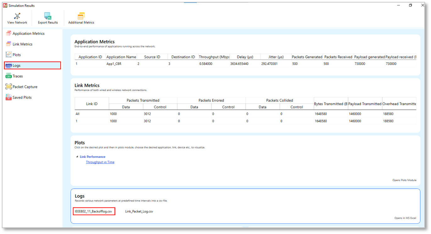
Figure-14: IEEE802_11_Backoff_Log.csv file highlighted in the Results window.

Figure-15: IEEE802_11_ Backoff_Log.csv file

Layer 2 (L2) Ethernet Switching

Layer 2 Switches have a MAC Address table that contains a MAC address and port number. Switches follow this simple algorithm for forwarding packets:

When a frame is received, the switch compares the SOURCE MAC address to the MAC address table. If the SOURCE is unknown, the switch adds it to the table along with the port number the packet was received on. In this way, the switch learns the MAC address and port of every transmitting device.
The switch then compares the DESTINATION MAC address with the table. If there is an entry, the switch forwards the frame out the associated port. If there is no entry, the switch sends the packet out all its ports, except the port that the frame was received on. This is termed as Flooding.
It does not learn the destination MAC until it receives a frame from that device

Spanning Tree Protocol

NetSim ethernet switches implement Spanning tree protocol to build a loop-free logical topology. This is always enabled and cannot be disabled.

Switch Port States

All switch ports in switches can be in one of the following states:

Blocking: A port that would cause a switching loop if it were active. No user data is sent or received over a blocking port.
Listening: The switch processes BPDUs and awaits possible new information that would cause it to return to the blocking state. It does not populate the MAC address table and it does not forward frames.
Learning: While the port does not yet forward frames, it does learn source addresses from frames received and adds them to the filtering database (switching database). It populates the MAC address table but does not forward frames.
Forwarding: A port receiving and sending data in Ethernet frames, normal operation.

It is recommended that the application start time is set to a value that is greater than the time it takes for the spanning tree protocol to complete (of the order of a 100s of milliseconds).

Model Limitations

The spanning protocol is only run at the beginning of simulation. If a link fails, the spanning protocol is not re-run.
If applications are started prior to completion of spanning tree protocol, then the MAC table created is not updated per the spanning tree protocol.
Jumbo Frames are not supported in NetSim Ethernet Protocol

Switch: GUI Parameters

Switch properties can be set by right clicking switch > Properties > Interface_1(ETHERNET).

Figure-16: Data Link Layer Properties of a Switch

The properties that can be set are:

Parameter	Type *	Range	Description
MAC ADDRESS	Fixed	Auto generated	The MAC address is a unique value associated with a network adapter. This is also known as hardware address or physical address. This is a 12-digit hexadecimal number (48 bits in length).
Buffer Size (MB)	Local	1-5	Buffer is the memory in a device which holds data packets temporarily. If the transmitting port is busy, incoming packets are stored in the buffer. NetSim models the buffer as an egress buffer and the range is 1 MB to 5MB per port of the switch.
STP Status	Fixed	TRUE	Spanning Tree Protocol is set to “True” in the Switches by default.
Switch Priority	Local	1-61440	This is the priority that can be assigned to the Switch. Priority is involved in deciding the root bridge for STP.
Switch ID	Local		Each switch has a unique ID for spanning tree calculation. The ID is derived by combining the priority and MAC address. Since a switch has a MAC address for each port, the least of the MAC addresses of the connected ports is taken while forming the unique ID.
Spanning Tree	Fixed	IEEE802.1D	The Spanning Tree Protocol (STP) ensures a loop-free topology for any bridged Ethernet local area network. The basic function of STP is to prevent bridge loops and the broadcast radiation that results from them. STP is standardized as IEEE 802.1D. As the name suggests, it creates a spanning tree within a network of connected layer-2 bridges (typically Ethernet switches) and disables those links that are not part of the spanning tree, leaving a single active path between any two network nodes.
STP Cost	Local	0-1000	Cost used by the switch to calculate spanning tree. The cost assigned to each port is based on its data rate.
Switching Mode	Local	Store Forward, Cut Through	Store and Forward: Forwarding takes place only after receipt of complete frame. This technique buffers the incoming frame and checks for errors. If no error is found it forwards the frame to the outgoing port, otherwise it discards the frame. Cut through: Switch forwards the incoming frames to its appropriate outgoing port immediately after receipt of destination address of the frame.
VLAN Status*	Local	TRUE, FALSE	To enable/disable VLAN

Table-21: Description of Datalink layer properties of switch parameter

*Requires license for Component 3 Advanced Routing and Switching

Open Shortest Path First (OSPF v2) Routing Protocol

OSPF Overview

OSPF is a link-state routing protocol. It is designed to be run internally to a single Autonomous System. Each OSPF router maintains an identical database describing the Autonomous System's topology. From this database, a routing table is calculated by constructing a shortest-path tree.

OSPF routes IP packets based solely on the destination IP address found in the IP packet header. IP packets are routed "as is" -- they are not encapsulated in any further protocol headers as they transit the Autonomous System. OSPF is a dynamic routing protocol. In NetSim, OSPF can detect topological changes in the AS (such as router interface failures) and calculate new loop-free routes after a period of convergence.

Each router maintains a database describing the Autonomous System's topology. This database is referred to as the link-state database. Each participating router has an identical database. Each individual piece of this database is a particular router's local state (e.g., the router's usable interfaces and reachable neighbors). The router distributes its local state throughout the Autonomous System by flooding.

All routers run the exact same algorithm, in parallel. From the link-state database, each router constructs a tree of shortest paths with itself as root. This shortest-path tree gives the route to each destination in the Autonomous System. The cost of a route is described by a single dimensionless metric.

OSPF Features

OSPF Messages – Hello, DD, LS Request, LS Update, LS Ack
Router LSA
The Neighbor Data structure features the following

Link state request list
DB summary list
Link state re-transmission list
Link state send list
Link state retransmission timer
Inactivity timer

Routing table
Shortest path tree
The Interface data structure features

Neighbor router list
Flood timer
Update LS list
Network LS timer
Delayed ack list

The Protocol data structure features

Interface list
Area list
Max age removal timer
SPF timer
Routing table

The Area Data structure features

Associated interface list
Router LSA list
Network LSA list
Router summary LSA list
Network summary LSA list
Max age list
Router LS timer
Shortest path list

The following can be logged during simulation

Hello log
SPF log
Common log
Debug logs – LSDB, RXList, RLSA, RCVLSU, LSULIST, Route

Excluded Features

The following features in OSPF have not been implemented - Multiple Areas, Network LSA, Router summary LSA, Network summary LSA, Authentication, Equal cost multipath, External AS, External routing information, Interface type – Broadcast, NBMA, Virtual, Point to multipoint

OSPF: GUI Parameters

OSPF properties can be set by right clicking on Router > Properties > Application layer see Figure-17.

Figure-17: Routing protocol properties of router.

The properties that can be set are:

Parameter	Type *	Range	Description
Version	Global	Fixed	OSPF Version 2 as per RFC 2328 for IPv4.
LSRefresh Time (s)	Global	Fixed	The maximum time between distinct originations of any particular Link State Advertisement (LSA). If the link state age field of one of the router’s self-originated LSAs reaches the value LSRefreshTime, a new instance of the LSA is originated, even though the contents of the LSA (apart from the LSA header) will be the same. The value of LSRefreshTime is set to 30 minutes.
LSA Maxage (s)	Global	Fixed	The maximum age that an LSA can attain. When an LSA's LS age field reaches MaxAge, it is reflooded in an attempt to flush the LSA from the routing domain. LSAs of age MaxAge are not used in the routing table calculation. The default value of MaxAge is set to 1 hour or 3600s
Increment Age (s)	Global	0 - 100	This is an internal variable of NetSim used for simulation purposes. This value decides how often to increase the age of the LSA in the OSPF LSA Lists. A small value will cause frequent updates and provide higher accuracy but may slow down simulation, and vice versa for a large value
Maxage removal Time (s)	Global	0 - 9999	This variable decides the time when the LSA is removed from the MaxAgeLSA List
Min LS Interval (s)	Global	Fixed	The minimum time between distinct originations of any particular LSA. The value of MinLSInterval is set to 5 seconds
SPF Calc Delay (ms)	Global	0 - 9999	If SPF calculation is triggered, then the router will wait for this duration before starting the calculation. This can be used for the router to take multiple updates into account
Flood Timer (ms)	Global	0 - 9999	The amount of time to wait before initializing the flood procedure. A random number between 0 to the set value will be chosen. The flood timer on/off is per the ISENDDELAYUPDATE variable setting
Advertise Self Interface	Global	True/False	This is reserved for future use. As of NetSim v12, this should always be true. This will be used when a point-to-multipoint link is connected to the interface, and when such links are connected this should be set to false
Send Delayed Update	Global	True/False	This variable can be set to true to delay sending the LSU. If set to true, then the delay would be per the flooding timer. Else the update is set immediately.

Table-22: Description of Application layer Routing protocol properties

*Global – Changes in all devices of similar type. Local – Only changes in current device

Transmission Control Protocol (TCP)

TCP overview

TCP is a connection-oriented, end-to-end reliable protocol designed to fit into a layered hierarchy of protocols which support multi-network applications. The TCP provides for reliable communication between host computers and connected computer communication networks. Very few assumptions are made as to the reliability of the communication protocols below the TCP layer. TCP assumes it can obtain a simple, potentially unreliable datagram service from the lower-level protocols. In principle, the TCP should be able to operate above a wide spectrum of communication systems ranging from wired to wireless to mobile communication.

The TCP fits into a layered protocol architecture just above a basic Internet Protocol which provides a way for the TCP to send and receive variable-length segments of information enclosed in IP packets. The IP packet provides a means for addressing source and destination TCPs in different networks. The IP protocol also deals with any fragmentation or reassembly of the TCP segments required to achieve transport and delivery through multiple networks and interconnecting gateways.

Application
TCP
IP
MAC
PHY

Table-23: Protocol Layering

TCP Features

The following features are implemented in TCP.

Three-way handshake (open/close)
Sequence Numbers
Slow start and congestion avoidance
Fast Retransmit/Fast Recovery
Selective Acknowledgement

Congestion Control Algorithms in TCP

The following congestion control algorithms are supported in NetSim.

Old Tahoe
Tahoe
Reno
New Reno
BIC
CUBIC

Limitations of TCP

Send and Receive buffers are infinite.

TCP: GUI parameters

The TCP parameters can be accessed by right clicking on a node and selecting Properties > Transport Layer.

Figure-18: Transport layer protocol properties of wired node

The properties that can be set are:

Parameter	Type *	Range	Description
Congestion Control Algorithm	Local	Old Tahoe, , Reno ,New Reno, Bic, Cubic	Congestion control algorithm is used to control the network congestion. Old Tahoe is the combination of slow start and congestion avoidance algorithm. The Fast-retransmit algorithm operating with Old Tahoe is known as the Tahoe. This algorithm works based on duplicate ack. When it receives three duplicate ack, which is the indication of segment loss, that segment will be retransmitted immediately without waiting for timeout. Reno implements fast recovery in case of three duplicate acknowledgements. New Reno improves retransmission during the fast-recovery phase of TCP Reno. BIC algorithm tries to find the maximum where to keep the window at for a long period of time, by using a binary search algorithm. CUBIC is an implementation of TCP with an optimized congestion control algorithm for high bandwidth networks with high latency.
Max SYN Retries	Local	1-10	Maximum number of TCP SYN ACK packets that can be retransmitted. The value should be in the range of 1 to 10.
Acknowledgement Type	Local	Delayed, Undelayed	If set to delayed, ACK response will be delayed improving network performance. If set to Un delayed, ACK will be sent immediately without delay.
MSS (bytes)	Local	64-1460	The maximum amount of data that a single message may contain. The MSS is the maximum data size and does not include the size of the header. MSS = MTU – (Network and Transport layer protocol headers).
Initial SSThreshold(bytes)	Local	5840-65535	The server-initial–ss-threshold should be in the range between 5840 and 65535 bytes.
Time Wait Timer(s)	Local	30-240	The Time wait timer default value is 120 seconds. The purpose of TIME-WAIT is to prevent delayed packets from one connection being accepted by a later connection.
Selective ACK	Local	TRUE, FALSE	In Selective Acknowledgement (SACK) mechanism, the receiving TCP sends back SACK packets to the sender informing the sender of data that has been received. The sender can then retransmit only the missing data segments.
Window Scaling	Local	TRUE, FALSE	The TCP window scaling option is to increase the receive window size allowed in Transmission Control Protocol above its former maximum value of 65,535 bytes.
Sack Permitted	Local	TRUE, FALSE	The SACK-permitted option is offered to the remote end during TCP setup as an option to an opening SYN packet. The SACK option permits selective acknowledgment of permitted data.
Timestamp Option	Local	TRUE, FALSE	TCP is a symmetric protocol, allowing data to be sent at any time in either direction. Therefore, timestamp echoing may occur in either direction. For simplicity and symmetry, we specify that timestamps always be sent and echoed in both directions. For efficiency, we combine the timestamp and timestamp reply fields into a single TCP Timestamps Option.

Table-24: Description of Transport layer protocol properties

TCP Performance Metrics

TCP Metrics table will be available in the Simulation Results dashboard if TCP is enabled in at least one device in the network. It provides the following information specific to TCP.

Parameter	Description
Source	It displays the name with ID of the source device which generates TCP packets
Destination	It displays the name with ID of the destination device which receives TCP packets
Local Address	It displays the local IP address with port number of the device present in source column
Remote Address	It represents the remote IP address with port number for the source and destination
Syn Sent	It is the number of syn packets sent by the source
Syn-Ack Sent	It is the number of syn ack packets sent by the destination
Segment Sent	It is the number of segments sent by a source
Segment Received	It is the number of segments received by a destination
Segment Retransmitted	It is the number of segments retransmitted by the source
Ack Sent	It is the number of acknowledgements sent by a source to destination in response to TCP syn ack and the number of acks sent by destination to source in response to the successful reception of data packet
Ack Received	It is the number of acknowledgements received by source in response to data packets and the number of acks received by destination in response to syn ack packet
Duplicate segment received	It is the number of duplicate segments received by destination
Out of order segment received	It is the number of out of order packets received by destination
Duplicate ack received	It is the number of duplicate acknowledgements received by source
Times RTO expired	It is the number of times RTO timer expired at source

Table-25: Parameter description of TCP Metrics table

TCP Reference Documents

RFC 793: TRANSMISSION CONTROL PROTOCOL
RFC 1122: Requirements for Internet Hosts -- Communication Layers
RFC 5681: TCP Congestion Control
RFC 3390: Increasing TCP's Initial Window
RFC 6298: Computing TCP's Retransmission Timer
RFC 2018: TCP Selective Acknowledgment Options
RFC 6582: The NewReno Modification to TCP's Fast Recovery Algorithm
RFC 6675: A Conservative Loss Recovery Algorithm Based on Selective Acknowledgment (SACK) for TCP
RFC 7323: TCP Extensions for High Performance
https://web.archive.org/web/20160505194415/http://netsrv.csc.ncsu.edu/export/cubic_a_new_tcp_2008.pdf
https://research.csc.ncsu.edu/netsrv/sites/default/files/bitcp.pdf
https://web.archive.org/web/20160528233754/http://netsrv.csc.ncsu.edu/export/hystart_techreport_2008.pdf

User Datagram Protocol (UDP)

UDP Overview

UDP (User Datagram Protocol) is a communication protocol that offers a limited amount of service when messages are exchanged between computers in a network that uses the Internet Protocol (IP). UDP uses the Internet Protocol to get a data unit (called a datagram) from one computer to another.

This protocol is transaction oriented, and delivery and duplicate protection are not guaranteed. Applications requiring reliable delivery of streams of data should use the Transmission Control Protocol (TCP).

UDP: GUI parameters

The UDP protocol can be set for an application by clicking on the Applications Transport Protocol option as shown below see Figure-19.

Figure-19: Application configuration window

UDP Performance Metrics

UDP Metrics table will be available in the Simulation Results dashboard if UDP is enabled in at least one device in the network. It provides the following information specific to UDP see Table-26.

Parameter	Description
Device Id	It is the Id of a device in which UDP is enabled
Local Address	It represents the IP address with port number of the local device (either source or destination)
Foreign Address	It represents the IP address with port number of the remote device (either source or destination)
Datagram sent	It is the total number of datagrams sent from the source
Datagram received	It is the total number of datagrams received at the destination

Table-26: Parameter description of UDP Metrics table

UDP Reference Documents

RFC 768: User Datagram Protocol

IP Protocol

IP Performance Metrics

IP Metrics table will be available in the Simulation Results dashboard if IP is enabled in at least one device in the network. It provides the following information specific to IP protocol:

Parameter	Description
Device Id	It displays the Id of the Layer 3 devices
Packet sent	It is the number of packets sent by a source, intermediate devices (Router or L3 switch)
Packet forwarded	It is the number of packets forwarded by intermediate devices (Router or L3 switch)
Packet received	It is the number of data packets received by destination, intermediate devices (routing packets (OSPF, RIP etc.) received by Routers)
Packet discarded	It is the number of data packets that are discarded after their TTL value expires.
TTL expired	Time-to-live (TTL) is a value in an Internet Protocol (IP) packet that tells a network router whether or not the packet has been in the network too long and should be discarded
Firewall blocked	It is the number of packets blocked by firewall at routers

Table-27: Parameter description of IP Metrics table

Buffering, Queueing and Scheduling

Buffers

Devices and their Interfaces with buffers that support queuing and scheduling algorithms are:

Router (WAN – Network Layer)
EPC (WAN – Network Layer)
6LOWPAN (WAN – Network Layer)
Satellite Gateway (WAN – Network Layer)

Queuing and scheduling in NetSim, works as follows:

The scheduler schedules packet transmission from the head-of-queue per the scheduling algorithm. FIFO algorithm uses a single queue while Priority, RR and WFQ use 4 queues (1 queue for each priority)
The buffer size is a user input. This buffer is not split among the various queues. At any point in time the cumulative size of all queues is the buffer fill.
The way in which the individual queues are filled up, is per the queuing algorithm selected (implemented in version 12.1)

The buffer is an egress buffer. The buffer size in Megabytes (MB), for each interface mentioned above is a user input. The options 8, 16, 32, 64, 128, 256, 512, 1024, 2048 and 4096 MB

Queuing

Drop Tail: The queue is filled up till the buffer capacity. When the queue is full if any packet arrives, it is dropped. The buffer size is a user input.

Random Early Detection (RED):

The queue is filled up till the average queue size is equal to minimum threshold, without dropping any packet.
Random packets are dropped when the average queue size is between minimum threshold and maximum threshold. The number of packets being dropped depends on the Max Probability value.
All packets are dropped when the average queue size is above maximum threshold.

User Inputs - Maximum threshold, minimum threshold and maximum probability.

\[Avg\ = \frac{t_{n}}{t_{n + 1}}\ \left( Avg - x_{n} \right) + x_{n}\]

\(Avg\) – Average Queue Size. \(Avg\) is initially 0

\(t_{n}\) – Time when n^th packet was added to the queue

\(t_{n + 1}\) – Current time which is the time when the (n+1)^th packet is added

\(x_{n}\) _– Size of n^th packet (B)

Packets are dropped if

\(No\ of\ Dropped\ Packets > \frac{Rand\ (0,1)}{P}\ \) where \(p = C_{1} \times Avg + C_{2}\)

\[C_{1} = \frac{Max\ Probability}{(Max\ Threshold - Min\ Threshold)}\]

\[C_{2} = \ \frac{Max\ Probability}{(Max\ Threshold - Min\ Threshold)} \times Min\ Threshold\]

Weighted Random Early Detection (WRED):

Please refer to RED explained earlier. This is modified as follows

There are different Max and Min threshold value for each type of priority, i.e. High, Medium, Normal, Low (The RED algorithm had only one set of Max and Min Threshold)
For the given threshold values of the packets, Random Early Detection (RED) algorithm is applied.

Reference Documents

Sally Floyd, Van Jacobson (1993). Random Early Detection Gateways for Congestion Avoidance. IEEE/ACM Transactions on Networking.

Queue Size: The queue depth can be obtained from the Event Trace or by modifying the protocol source code. To obtain it from the event trace, an MS Excel script would need to be written to filter by node, and at different points of time, add the number of APP-OUT events and subtract the number of TRANSPORT-OUT events. Note that deeper issues such as segmentation etc. will need to be handled appropriately based on the way the application and transport layer interact.

Scheduling

First In First Out (FIFO): Packets are scheduled according to their arrival time in the queue. Hence, first packet in queue is scheduled first.

Priority: NetSim supports 4 priority queues namely High, Medium, Normal and Low. With this scheduling, first all packets in the High priority queue are served, and then those in Medium, then in normal and finally those packets in the low priority queue. Note that this could lead to situations where only higher priority packets are served and lower priority packets are never served.

Round Robin: Packets from all the 4 priorities are served in circular order. When packet arrives, they are stored in the corresponding priority list

Weighted Fair Queuing (WFQ): When packet arrive, they are stored in corresponding list according to priority. Packets are served in order of maximum weight of the priority list. In NetSim WFQ is approximated as:

\(Weight = (Number\ of\ packets\ in\ Queue) \times Priority\) where

\[Priority = 1,\ 2,\ 3\ or\ 4\]

1 - Low priority, 2 - Normal, 3 – Medium, 4 - High

Early Deadline First (EDF): Packets are added in the queue as they arrive. While dequeuing the packets with earliest deadline are served first. The packets which have exceeded deadline are dropped.

\[Deadline = Max\ Latency - Packet\ Creation\ Time\]

Max Latency with respect to quality of service (QoS) of the packet is a user input

Links

Modeling Error in Wired Links

The error rates in NetSim wired links are based on a standard error measurement unit called BER or Bit Error Rate. BER represents the ratio of errored bits to total bits.

The BER value can be set by the user. A typical value of BER, say \(1 \times 10^{- 6}\), which equals 0.000001, means that 1 bit is in error for every one-million bits transmitted. It is important to note that Bit Error Rate is not equal to Packet error rate. (PER)

\[PER = 1 - (1 - BER)^{L}\ where\ L\ is\ the\ packet\ length\ in\ bits\]

For BER values less than 0.001, this is mathematically approximated in NetSim as

\[PER = BER*L\]

IP Addressing in NetSim

When you create a network using the GUI, NetSim will automatically configure the IP address to the devices in the scenario. Consider the following scenarios:

If you create a network with two wired nodes and L2_Switch, the IP addresses are assigned as 192.168.0.2 and 192.168.0.3 for the two wired nodes. The default subnet mask is assigned to be 255.255.0.0. It can be edited to 255.0.0.0 (Class A) or 255.255.255.0 (Class C) subnet masks. Both the nodes are in the same network (192.168.0.0).

Similarly, if you create a network with a router and two wired nodes, the IP addresses are assigned as 192.168.0.1 and 192.169.0.1 for the two wired nodes. The subnet mask is default as in above case, i.e., 255.255.0.0. The IP address of the router is 192.168.0.1 and 192.169.0.1 respectively for the two interfaces. Both the nodes are in different networks (192.168.0.0 and 192.169.0.0) in this case.

The same logic is extended as the number of devices increases.