Featured Examples
Sample configuration files for all networks are available in the Examples Menu in NetSim Home Screen. These files provide examples on How NetSim can be used – the parameters that can be changed and the typical effect it has on performance.
802.11n MIMO
Open NetSim, Select Examples -> Internetworks -> Wi-Fi -> 802.11n-MIMO then click on the tile in the middle panel to load the example shown in Figure-1.
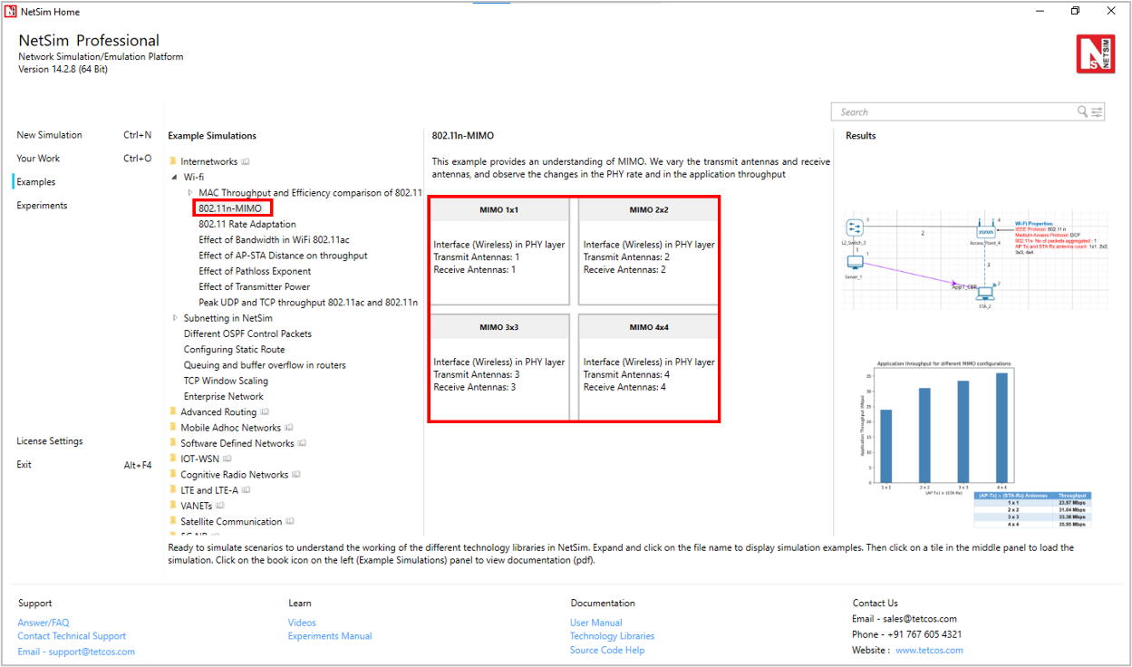
Figure-1: List of scenarios for the example of 802.11n-MIMO
The following network diagram illustrates what the NetSim UI displays when you open the example configuration file for 802.11n-MIMO.
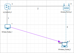
Figure-2: Network setup for studying the 802.11n-MIMO
Network Settings
Set grid length as 60m × 30m from grid setting property panel on the right. This needs to be done before any device is placed on the grid.
Distance between AP and Wireless node is 20m.
Set DCF as the medium access layer protocol under datalink layer properties of access point and wireless node (STA). To configure any properties in the nodes, click on the node, expand the property panel on the right side, and change the properties as mentioned in the below steps.
In Interface (Wireless) properties of physical layer, WLAN Standard is set to 802.11n and No. of Tx and Rx Antennas is set to 1 in both Access Point and STA.
Click on wireless link and expand property panel on the right and set the Channel Characteristics a Pathloss, Path Loss Model a Log Distance and Path loss Exponent a 3. (Wireless Link Properties).
Configure CBR application between server and STA by clicking on the set traffic tab from the ribbon at the top. Click on created application and expand the application property panel on the right and set transport protocol to UDP, packet size to 1460 B and Inter arrival time as 233 µs.
Simulate for 10 sec and check the throughput.
Go back to the scenario and increase the Number of Tx and Rx Antenna \(1 \times 1,\) \(\ 2 \times 2,\ \ 3 \times 3\), \(\ 4 \times 4\) respectively and check the throughput in the results window.
Results and Discussion
Number of Tx and Rx Antenna |
Throughput |
|---|---|
1 x 1 |
23.97 Mbps |
2 x 2 |
31.04 Mbps |
3 x 3 |
33.38 Mbps |
4 x 4 |
35.95 Mbps |
Table-1: Number of Tx and Rx Antenna vs. Throughput
MIMO is a method for multiplying the capacity of a radio link using multiple transmit and receive antennas. Increasing the Transmitting Antennas and Receiving Antennas in PHY Data rate (link capacity) and hence leads to an increase in application throughput.
Plot
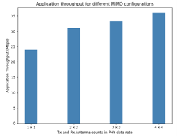
Figure-3: Plot of Tx and Rx Antenna counts vs Throughput
Effect of Bandwidth in Wi-Fi 802.11ac
Effect of Bandwidth
Open NetSim and Select Examples > Internetworks > Wi-Fi > Effect of bandwidth in Wi-Fi 802.11ac then click on the tile in the middle panel to load the example as shown in Figure-4.

Figure-4: List of scenarios for the example of effect of bandwidth in Wi-Fi 802.11ac
The following network diagram illustrates what the NetSim UI displays when you open the example configuration file as shown Figure-5.

Figure-5: Network setup for studying the effect of bandwidth in Wi-Fi 802.11ac
Network Settings
Set grid length to 60m \(\times\) 30m from the grid setting property panel on the right. This needs to be done before any device is placed on the grid.
Set 802.11ac standard and Bandwidth to 20MHz under Wireless Interface->Physical Layer properties of the access point and wireless node. To configure any properties in the nodes, click on the node, expand the property panel on the right side, and change the properties as mentioned in the below steps.
Set DCF as the medium access layer protocol under Wireless Interface-> datalink layer properties of access point and wireless node
Set transmitter power as 40mW under Wireless Interface ->Transmitter Power properties of the access point and wireless node.
Click on wireless link and open property panel on the right and set the Channel Characteristics: No pathloss in wireless link properties.
Similarly, set Bit Error rate and Propagation delay to zero under wired link properties
Configure CBR application between server and STA by clicking on the set traffic tab from the ribbon at the top. Click on created application and expand the application property panel on the right and set transport protocol to UDP, packet size to 1460 B and Inter arrival time as 116 µs (Generation rate is 100.6 Mbps)
Generation rate is set to 100 Mbps in application properties (Packet Size = 1460 Bytes, Interarrival time = 116.8 microseconds). Generation rate can be calculated by using the formula below:
Run simulation for 10s and see application throughput in the results window.
Go back to the scenario and increase the Bandwidth 20 to 40, 80, 160 respectively and check the throughput in the results window.
Analytical Model
The average time to transmit a packet comprises of
DIFS
Backoff duration
Data packet transmission time
SIFS
MAC ACK transmission time
The timing diagram is as shown below Figure-6.

Figure-6: Timing diagram for WLAN
The Average throughput can be calculated by using the formula below:
Where,
Similarly calculate throughput theoretically for other samples by changing bandwidth and compare with simulation throughput. Users can get the data rate by using the formula given below:
𝑃ℎ𝑦 𝑟𝑎𝑡𝑒 (802.11ac) = 𝑃ℎ𝑦_𝑙𝑎𝑦𝑒𝑟_𝑝𝑎𝑦𝑙𝑜𝑎𝑑 ∗ 8/(𝑝ℎ𝑦 𝑒𝑛𝑑 𝑡𝑖𝑚𝑒 − 𝑝ℎ𝑦 𝑎𝑟𝑟𝑖𝑣𝑎𝑙𝑡𝑖𝑚𝑒 − 44)
Results and Discussion
Bandwidth (MHz) |
Analytical Estimate of Throughput (Mbps) |
Simulation Throughput (Mbps) |
|---|---|---|
20 |
22.70 |
22.81 |
40 |
33.77 |
33.94 |
80 |
43.39 |
43.67 |
160 |
49.35 |
49.78 |
Table-2: Result comparison of different bandwidth vs. Analytical Estimate of Throughput and Simulation Throughput
One can observe that there is an increase in throughput as we increase the bandwidth from 20MHz to 160MHz.
Plot

Figure-7: Plot of Bandwidth vs Throughput
Factors affecting WLAN PHY Rate
The examples explained in this section focuses on the factors which affect the PHY Rate/Link Throughput of 802.11 based networks:
Transmitter power (More Tx power leads to higher throughput)
Channel Path loss (Higher path loss exponent leads to lower throughput)
Receiver sensitivity (Lower Rx sensitivity leads to higher throughput)
Distance (Higher distance between nodes leads to lower throughput)
Effect of AP-STA Distance on throughput
Open NetSim and Select Examples > Internetworks > Wi-Fi > Effect of AP STA Distance on throughput then click on the tile in the middle panel to load the example as shown in Figure-8.

Figure-8: List of scenarios for the example effect of AP-STA distance on throughput
The following network diagram illustrates what the NetSim UI displays when you open the example configuration file see Figure-9.

Figure-9: Network setup for studying the Effect of AP-STA Distance on throughput.
As the distance between two devices increases the received signal power reduces as propagation loss increases with distance. As the received power reduces, the underlying PHY rate of the channel drops.
Network Settings
Set grid length to 120m x 60m grid setting property panel on the right. This needs to be done before the any device is placed on the grid.
Distance between Access Point and the Wireless Node is set to 5m
Set DCF as the medium access layer protocol under datalink layer properties of access point and wireless node. To configure any properties in the nodes, click on the node, expand the property panel on the right side, and change the properties as mentioned in the below steps.
WLAN Standard is set to 802.11ac and No. of Tx and Rx Antenna is set to 1 in access point and No. of Tx is 1 and Rx Antenna is set to 1 in wireless node (Right-Click Access Point or Wireless Node > Properties > Interface Wireless > Transmitting Antennas and Receiving Antennas) and Bandwidth is set to 20 MHz in both Access-point and wireless-node Transmitter Power set to 100mW in both Access-point and wireless-node.
Wired Link speed is set to 1Gbps and propagation delay to 10 µs in wired links.
Channel Characteristics: Pathloss, Path loss model: Log distance, Path loss exponent: 3.5.
Configure an application between any two nodes by selecting a CBR application from the Set Traffic tab in the ribbon on the top. Click on created application and expand the application property panel on the right and set transport protocol to UDP, packet size to 1460 B and Inter arrival time to 116.8 µs.
Application Generation Rate: 100 Mbps (Packet Size: 1460, Inter Arrival Time: 116.8 µs)
Run the simulation for 10s.
Go back to the scenario and increase the distance as per result table and run simulation for 10s.
Results
Distance (m) |
Throughput (Mbps) |
|---|---|
5 |
22.81 |
10 |
21.61 |
15 |
17.87 |
20 |
14.70 |
25 |
12.49 |
30 |
9.56 |
35 |
5.63 |
40 |
0 |
Table-3: Result comparison of different distance vs. throughput
Plot

Figure-10: Plot of Distance vs Throughput
Effect of Pathloss Exponent
Open NetSim and Select Examples > Internetworks > Wi-Fi > Effect of Pathloss Exponent then click on the tile in the middle panel to load the example as shown in Figure-11.

Figure-11: List of scenarios for the example of effect of pathloss exponent
The following network diagram illustrates what the NetSim UI displays when you open the example configuration file as shown Figure-12.
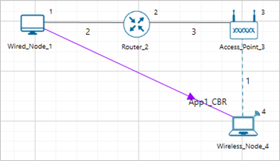
Figure-12: Network setup for studying the effect of pathloss exponent
Path Loss or Attenuation of RF signals occurs naturally with distance. Losses can be increased by increasing the path loss exponent (η). This option is available in channel characteristics. Users can compare the results by changing the path loss exponent (η) value.
Network Settings
Set grid length to 80m x 40m from grid setting property panel on the right. This needs to be done before any device is placed on the grid.
Distance between Access Point and the Wireless Node is set to 20m
Set DCF as the medium access layer protocol under datalink layer properties of access point and wireless node. To configure any properties in the nodes, click on the node, expand the property panel on the right side, and change the properties as mentioned in the below steps.
WLAN Standard is set to 802.11ac and No. of Tx and Rx Antenna is set to 1 in both access point and wireless node and Bandwidth is set to 20 MHz in both Access-point and wireless-node and Transmitter Power set to 100mW in both Access-point and wireless-node.
Click on the wireless link and open property panel on the right and set the Channel Characteristics: Path Loss Only, Path Loss Model: Log Distance, Path Loss Exponent: 2
Configure an application between any two nodes by selecting a CBR application from the Set Traffic tab in the ribbon on the top. Click on created application and expand the application property panel on the right and set transport protocol to UDP, packet size to 1460 B and Inter arrival time to 116 µs.
Run simulation for 10s.
Go back to the scenario and increase the Path Loss Exponent from 2 to 2.5, 3, 3.5, 4, and 4.5 respectively and Run simulation for 10s.
Results
Path loss Exponent |
Throughput (Mbps) |
|---|---|
2.0 |
22.81 |
2.5 |
21.61 |
3.0 |
20.04 |
3.5 |
14.70 |
4.0 |
9.56 |
4.5 |
0 |
Table-4: Result comparison of different pathloss exponent value vs. throughput
Plot

Figure-13: Plot of Path loss Exponent vs Throughput
Effect of Transmitter power
Open NetSim and Select Examples->Internetworks->Wi-Fi-> Effect of Transmitter Power then click on the tile in the middle panel to load the example as shown in Figure-14.

Figure-14: List of scenarios for the example of effect of transmitter power
The following network diagram illustrates what the NetSim UI displays when you open the example configuration file see Figure-15.

Figure-15: Network setup for studying the effect of transmitter power
Increase in transmitter power increases the received power when all other parameters are constant. Increased received power leads to higher SNR and hence higher PHY Data rates, lesser error and higher throughputs.
Network Settings
Set grid length to 120m x 60m from grid setting property panel on the right. This needs to be done before any device is placed on the grid.
Distance between Access Point and the Wireless Node is set to 35m
Set transmitter power to 100mW under Interface Wireless > Physical layer properties of Access point. To configure any properties in the nodes, click on the node, expand the property panel on the right side, and change the properties as mentioned in the below steps.
Set DCF as the medium access layer protocol under datalink layer properties of access point and wireless node.
Click on wireless link and open property panel on the right and set the Channel Characteristics: Path Loss Only, Path Loss Model: Log Distance, Path Loss Exponent: 3.5
Configure CBR application between server and STA by clicking on the set traffic tab from the ribbon at the top. Click on created application and expand the application property panel on the right and set transport protocol to UDP, packet size to 1460 B and Inter arrival time to 1168 µs
Run the simulation for 10s
Go back to the scenario and decrease the Transmitter Power to 60, 40, 20 and 10 respectively and run simulation for 10s. See that, there is a decrease in the Throughput gradually.
Results
Transmitter Power (mW) |
Throughput (Mbps) |
Phy Rate (Mbps) |
|---|---|---|
100 |
5.94 |
11 |
60 |
3.79 |
5 |
40 |
1.67 |
2 |
20 |
0.89 |
1 |
10 |
0.0 |
0 |
Table-5: Result comparison of different transmitter power vs. throughput
Plot

Figure-16: Transmitter power vs Throughput
Open NetSim, Select Examples->Internetworks-> Wi-Fi -> Peak UDP and TCP throughput 802.11ac and 802.11n then click on the tile in the middle panel to load the example as shown Figure-17.

Figure-17: List of scenarios for the example of Peak UDP and TCP throughput 802.11ac and 802.11n
The following network diagram illustrates what the NetSim UI displays when you open the example configuration file as shown Figure-18.

Figure-18: Network setup for studying the Peak UDP and TCP throughput 802.11ac and 802.11n
IEEE802.11n
Network Settings
Set the following property in access point and wireless node as shown in below given Table-6. To configure any properties in the nodes, click on the node, expand the property panel on the right side, and change the properties as follows.
Interface Parameters |
|
|---|---|
Physical Layer |
|
Standard |
IEEE802.11n |
No. of Frames to aggregate |
64 |
Transmitter Power |
100mW |
Frequency Band |
5 GHz |
Bandwidth |
40 MHz |
Standard Channel |
36 (5180MHz) |
Guard Interval |
400ns |
Antenna |
|
Antenna height |
1m |
Antenna Gain |
0 |
Transmitting Antennas |
4 |
Receiving Antennas |
4 |
Datalink Layer |
|
Rate Adaptation |
False |
Short Retry Limit |
7 |
Buffer Size |
100 MB |
Long Retry Limit |
4 |
Dott11_RTSThreshold |
3000 bytes |
Medium Access Protocol |
DCF |
Table-6: Detailed Network Parameters for IEEE802.11n
To configure wired and wireless link properties, click on link, expand the property panel on the right and set wired link properties as shown below.
Uplink speed and Downlink speed (Mbps)- 1000 Mbps.
Uplink BER and Downlink BER – 0.
Uplink and Downlink Propagation Delay(µs) – 10.
The Channel Characteristics were set as No pathloss in wireless link properties.
Configure CBR application from source node (Wired Node) to destination node (Wireless Node) by clicking on the set traffic tab from the ribbon at the top. Click on created application, expand the application property panel on the right and set the following properties.
Application Properties |
|
|---|---|
App1 CBR |
|
Packet Size (Byte) |
1460 |
Inter Arrival Time (µs) |
11.6 |
Transport Protocol |
UDP |
Table-7: Application Parameters
Run simulation for 5 sec. After simulation completes go to metrics window and note down throughput value from application metrics.
Go Back to 802.11n UDP scenario and change transport protocol to TCP, window scaling is set to true and scale shift count set to 5 in the transport layer of wired node and wireless node for the other sample (i.e 802.11n TCP), run the simulation for 5 sec and note down throughput value from application metrics.
Results
Transport Protocol |
Throughput (Mbps) |
|---|---|
UDP |
443.16 |
TCP |
347.51 |
Table-8: Results comparison of TCP and UDP throughputs for IEEE802.11n
Plot

Figure-19: Plot of Throughput (Mbps) Vs. Transport Protocol for IEEE802.11n
IEEE802.11ac
Network Settings
Set the following property in access point and wireless node as shown in below given table:
Interface Parameters (Wireless and Access point) |
|
|---|---|
Data link layer |
|
Rate Adaptation |
False |
Short Retry Limit |
7 |
Long Retry Limit |
4 |
Dott11_RTSThreshold |
3000bytes |
Medium Access Protocol |
DCF |
Physical layer |
|
Standard |
IEEE802.11ac |
No. of Frames to aggregated |
1024 |
Transmitter Power |
100mW |
Frequency Band |
5 GHz |
Bandwidth |
160 MHz |
Standard Channel |
36 (5180MHz) |
Guard Interval |
400ns |
Antenna |
|
Antenna height |
1m |
Antenna Gain |
0 |
Transmitting Antennas |
8 |
Receiving Antennas |
8 |
Access Point |
|
Buffer Size |
100MB |
Table-9: Detailed Network Parameters for IEEE802.11ac
To configure wired and wireless link properties, click on link, expand the property panel on the right and set wired link properties as shown below.
Uplink speed and Downlink speed (Mbps) - 10000 Mbps.
Uplink BER and Downlink BER – 0.
Uplink and Downlink Propagation Delay(µs) – 10.
The Channel Characteristics were set as No pathloss in wireless link properties.
Configure CBR application from source node (Wired Node) to destination node (Wireless Node) by clicking on the set traffic tab from the ribbon at the top. Click on created application, expand the application property panel on the right and set the following properties.
Application Properties |
|
|---|---|
App1_CBR |
|
Packet Size (Byte) |
1450 |
Inter Arrival Time (µs) |
1.93 |
Transport Protocol |
UDP |
Table-10: Application Parameters
Run simulation for 10 sec. After simulation completes go to metrics window and note down throughput value from application metrics.
Go Back to the 802.11ac UDP scenario and change transport protocol to TCP, window scaling is set to true and scale shift count set to 5 in the transport layer of wired node and wireless node for the other sample (i,e 802.11ac TCP), run the simulation for 10 sec and note down throughput value from application metrics.
Results
Transport Protocol |
Throughput (Mbps) |
|---|---|
UDP |
5589.08 |
TCP |
3397.16 |
Table-11: Results comparison of TCP and UDP throughputs for IEEE802.11ac
Plot
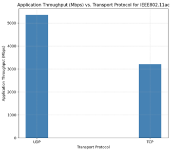
Figure-20: Plot of Throughput (Mbps) Vs. Transport Protocol for IEEE802.11ac
MAC Throughput and Efficiency comparison of 802.11 Legacy vs. HT protocols
This example is based on Part II, Section 9 by E. Perahia and R. Stacey, from 'Next Generation Wireless LANs,' published by Cambridge University Press.
Network Scenario

Figure-21: Network Scenario consists of 1 Wired Node, 1 Switch, 1 AP and 1 STA.
Part I: Legacy
Steps:
Create a scenario with 1 Wired Node,1 L2 Switch, 1 Access Point and 1 STA as shown in Figure-21.
Click on Wired link and expand property panel on the right and set the Wired Link Properties, Uplink and Downlink Speed as 1000 Mbps, Bit Error Rate to 0, and Propagation Delay to 0 µs.
Click on Wireless link and expand property panel and configure the Wireless Link Properties as shown below.
Wireless Link Parameters |
|
|---|---|
Channel Characteristics |
Pathloss |
Pathloss Model |
Log Distance |
Pathloss Exponent |
2 |
Table-12: Wireless Link Properties.
Configure the CBR application between two nodes by clicking on the set traffic tab from the ribbon at the top, selecting Source ID as 1 and Destination ID as 4. Click on the created application and set the transport protocol to UDP with a Packet Size as 1460 Bytes and Inter Arrival Time as 194.66 µs.
Configure the Access Point and Wireless Node properties as shown below.
Interface (Wireless) 🡪 Datalink Layer |
|
|---|---|
Rate Adaptation |
False |
RTS Threshold |
4692480 Bytes |
Long Retry Limit |
4 |
Medium Access Protocol |
DCF |
Buffer Size(Access Point) |
100 MB |
Interface (Wireless) 🡪 Physical Layer |
|
Standard |
IEEE802.11g |
Transmitter Power |
100mW |
Frequency Band |
2.4 GHz |
Bandwidth |
20MHz |
Standard Channel |
1 (2412MHz) |
Antenna |
|
Antenna height |
0 m |
Antenna Gain |
0 |
Table-13: Network Configuration for IEEE802.11g.
Go to Configure Reports Tab > Click on Plots > On the Right-Hand Side Plots Tab > Expand Network Logs > Enable IEEE 802.11 Radio Measurements Log.

Figure-22: Enabling IEEE 802.11 Radio Measurements logs.
Run the Simulation for 10 seconds.
Similarly vary the distance between Access Point and Wireless Nodes, Note down the results such as MCS and Throughput (Mbps) by filtering the control packet type to data packets in IEEE 802.11 Radio Measurements Log.
Part II: High Throughput (HT)
Case 1: High-throughput 802.11n with a 20MHz bandwidth
Consider the same above Legacy network case.
Configure the CBR application between two nodes by clicking on the set traffic tab from the ribbon at the top, selecting Source ID as 1 and Destination ID as 4. Click on the created application and set the transport protocol to UDP with a Packet Size as 1460 Bytes and Inter Arrival Time as 57.14 µs.
Configure the Access Point and Wireless Node properties as shown below.
Interface (Wireless) 🡪 Datalink Layer |
|
|---|---|
Rate Adaptation |
False |
RTS Threshold |
4692480 Bytes |
Long Retry Limit |
4 |
Medium Access Protocol |
DCF |
Buffer Size(Access Point) |
100 MB |
Interface (Wireless) 🡪 Physical Layer |
|
Standard |
IEEE802.11n |
No. of Frames aggregated |
1 |
Transmitter Power |
100mW |
Frequency Band |
2.4 GHz |
Bandwidth |
20MHz |
Standard Channel |
1 (2412MHz) |
Guard Interval |
400 ns |
Antenna |
|
Antenna height |
0 m |
Antenna Gain |
0 |
TX Antenna Count |
1 |
RX Antenna Count |
1 |
Table-14: Network Configuration for IEEE802.11n.
Go to Configure Reports tab and enable packet trace and click on Plots > on the right-hand side Tab > expand Network Logs > enable IEEE 802.11 Radio Measurements Figure-22.
Run the simulation for 10 seconds.
Similarly vary Antenna Count and the distance between Access Point and Wireless Node as shown in the Table-16.
Run the simulation for 10 seconds. Record the results such as MCS from IEEE 802.11 Radio Measurements Log and Throughput (Mbps) from the Application Metrics.
Change the No. of Frames Aggregated to 64, repeat the Step 6 and 7 again. The similar settings are done in 802.11n-20MHz-Frames-Aggregation:64 sample
Note:
In NetSim, we have provided one sample for each case. For additional samples, you need to run simulations with varying values for antenna count and distance as mentioned in Table-15 , Table-16 and Table-17.
In the IEEE 802.11 Radio Measurements Log, filter the Control Packet Type to App1_CBR to note down the MCS value for all cases.
Case 2: High-throughput 802.11n with a 40MHz bandwidth
For the same case 1, change the bandwidth to 40MHz, No. of Frames Aggregated to 1 and rerun the sample by varying Antenna Count and the distance between Access Point and Wireless Node as shown in the Table-17.
Run the Simulation for 10 seconds. Record the results such as MCS from IEEE 802.11 Radio Measurements Log and Throughput (Mbps) from the Application Metrics.
Again, change the No. of Frames Aggregated to 64. Vary Antenna Count and the distance between Access Point and Wireless Node as shown in the Table 4 17.The similar settings are done in 802.11n 40MHz Frames Aggregation 64 sample.
Run the Simulation for 10 seconds. Record the results such as MCS from IEEE 802.11 Radio Measurements Log and Throughput (Mbps) from the Application Metrics.
MAC Efficiency:
MAC efficiency is defined as
\(Efficiency\ (\%) = \frac{Throughput\ (Mbps)}{PHY\ Rate\ (Mbps)}\ \times 100\)
Note:
The PHY Rate and Receiver Sensitivity values are taken from the IEEE 802.11 (Wi-Fi) Standard as follows:
IEEE 802.11g: PHY Rate and Receiver Sensitivity are specified in Table 17-4 and Table 17-18 of the IEEE 802.11-2020 standard.
IEEE 802.11n: PHY Rate is specified in Tables 19-27 to 19-34, and Receiver Sensitivity is specified in Table 19-23 of the IEEE 802.11-2020 standard.
Results
802.11g (Legacy):
Standard |
Distance (m) |
MCS |
RX Sensitivity (dBm) |
PHY Rate (Mbps) |
Throughput (Mbps) |
Efficiency (%) |
|---|---|---|---|---|---|---|
802.11 g |
166 |
7 |
-65 |
54 |
29.21 |
54 |
196 |
6 |
-66 |
48 |
27.31 |
57 |
|
301 |
5 |
-70 |
36 |
22.78 |
63 |
|
496 |
4 |
-74 |
24 |
17.11 |
71 |
|
691 |
3 |
-77 |
18 |
13.70 |
76 |
|
871 |
2 |
-79 |
12 |
9.80 |
82 |
|
1096 |
1 |
-81 |
9 |
7.63 |
85 |
|
1111 |
0 |
-82 |
6 |
5.29 |
88 |
Table-15: Results of 802.11g (Legacy).
Case 1: 802.11n 20 MHz:
Aggregation = 1 |
Aggregation = 64 |
|||||||
|---|---|---|---|---|---|---|---|---|
Distance (m) |
Antenna Count |
MCS |
RX Sensitivity (dBm) |
PHY Rate (Mbps) |
Throughput (Mbps) |
Efficiency (%) |
Throughput (Mbps) |
Efficiency (%) |
151 |
1x1 |
7 |
-64 |
72.2 |
23.99 |
33 |
66.88 |
93 |
166 |
1x1 |
6 |
-65 |
65 |
23.11 |
36 |
60.38 |
93 |
196 |
1x1 |
5 |
-66 |
57.8 |
22.08 |
38 |
53.84 |
93 |
301 |
1x1 |
4 |
-70 |
43.3 |
19.47 |
45 |
40.56 |
94 |
496 |
1x1 |
3 |
-74 |
28.9 |
15.77 |
55 |
27.23 |
94 |
691 |
1x1 |
2 |
-77 |
21.7 |
13.25 |
61 |
20.50 |
94 |
871 |
1x1 |
1 |
-79 |
14.4 |
10.00 |
69 |
13.64 |
95 |
886 |
1x1 |
0 |
-82 |
7.2 |
5.79 |
80 |
6.84 |
95 |
151 |
2x2 |
7 |
-64 |
144.4 |
31.05 |
0 |
130.67 |
90 |
166 |
2x2 |
6 |
-65 |
130 |
30.29 |
22 |
118.25 |
91 |
196 |
2x2 |
5 |
-66 |
115.6 |
29.39 |
23 |
105.69 |
91 |
301 |
2x2 |
4 |
-70 |
86.7 |
26.99 |
25 |
80.08 |
92 |
496 |
2x2 |
3 |
-74 |
57.8 |
23.21 |
31 |
53.94 |
93 |
691 |
2x2 |
2 |
-77 |
43.3 |
20.34 |
40 |
40.62 |
94 |
871 |
2x2 |
1 |
-79 |
28.9 |
16.34 |
47 |
27.26 |
94 |
886 |
2x2 |
0 |
-82 |
14.4 |
10.23 |
57 |
13.65 |
95 |
151 |
3x3 |
7 |
-64 |
216.7 |
33.37 |
71 |
191.18 |
88 |
166 |
3x3 |
6 |
-65 |
195 |
32.78 |
0 |
173.32 |
89 |
196 |
3x3 |
5 |
-66 |
173.3 |
32.08 |
15 |
155.18 |
90 |
301 |
3x3 |
4 |
-70 |
130 |
30.13 |
17 |
118.21 |
91 |
496 |
3x3 |
3 |
-74 |
86.7 |
26.87 |
19 |
80.06 |
92 |
691 |
3x3 |
2 |
-77 |
65 |
24.24 |
23 |
60.49 |
93 |
871 |
3x3 |
1 |
-79 |
43.3 |
20.27 |
31 |
40.61 |
94 |
886 |
3x3 |
0 |
-82 |
21.7 |
13.62 |
37 |
20.52 |
95 |
151 |
4x4 |
7 |
-64 |
288.9 |
35.96 |
47 |
249.53 |
86 |
166 |
4x4 |
6 |
-65 |
260 |
35.44 |
63 |
226.67 |
87 |
196 |
4x4 |
5 |
-66 |
231.1 |
34.81 |
12 |
203.44 |
88 |
301 |
4x4 |
4 |
-70 |
173.3 |
33.07 |
14 |
155.54 |
90 |
496 |
4x4 |
3 |
-74 |
115.6 |
30.07 |
15 |
105.83 |
92 |
691 |
4x4 |
2 |
-77 |
86.7 |
27.56 |
19 |
80.15 |
92 |
871 |
4x4 |
1 |
-79 |
57.8 |
23.62 |
26 |
53.97 |
93 |
886 |
4x4 |
0 |
-82 |
28.9 |
16.54 |
32 |
27.27 |
94 |
Table-16: Results for 802.11n with 20 MHz Bandwidth varying Distance, MCS and Phy Rate.
Case 2: 802.11n 40 MHz:
Aggregation = 1 |
Aggregation = 64 |
|||||||
|---|---|---|---|---|---|---|---|---|
Distance (m) |
Antenna Count |
MCS |
RX Sensitivity (dBm) |
PHY Rate (Mbps) |
Throughput (Mbps) |
Efficiency (%) |
Throughput (Mbps) |
Efficiency (%) |
106 |
1x1 |
7 |
-61 |
150 |
30.71 |
20 |
135.29 |
90 |
121 |
1x1 |
6 |
-62 |
135 |
29.99 |
22 |
122.43 |
91 |
136 |
1x1 |
5 |
-63 |
120 |
29.14 |
24 |
109.44 |
91 |
211 |
1x1 |
4 |
-67 |
90 |
26.86 |
30 |
82.96 |
92 |
346 |
1x1 |
3 |
-71 |
60 |
23.23 |
39 |
55.92 |
93 |
496 |
1x1 |
2 |
-74 |
45 |
20.46 |
45 |
42.17 |
94 |
616 |
1x1 |
1 |
-76 |
30 |
16.53 |
55 |
28.28 |
94 |
631 |
1x1 |
0 |
-79 |
15 |
10.47 |
70 |
14.21 |
95 |
106 |
2x2 |
7 |
-61 |
300 |
36.17 |
12 |
258.20 |
86 |
121 |
2x2 |
6 |
-62 |
270 |
35.66 |
13 |
234.62 |
87 |
136 |
2x2 |
5 |
-63 |
240 |
35.06 |
15 |
210.66 |
88 |
211 |
2x2 |
4 |
-67 |
180 |
33.35 |
19 |
161.20 |
90 |
346 |
2x2 |
3 |
-71 |
120 |
30.40 |
25 |
109.70 |
91 |
496 |
2x2 |
2 |
-74 |
90 |
27.93 |
31 |
83.12 |
92 |
616 |
2x2 |
1 |
-76 |
60 |
24.02 |
40 |
55.99 |
93 |
631 |
2x2 |
0 |
-79 |
30 |
16.92 |
56 |
28.29 |
94 |
106 |
3x3 |
7 |
-61 |
450 |
37.16 |
8 |
368.53 |
82 |
121 |
3x3 |
6 |
-62 |
405.5 |
36.81 |
9 |
336.73 |
83 |
136 |
3x3 |
5 |
-63 |
360 |
36.36 |
10 |
303.27 |
84 |
211 |
3x3 |
4 |
-67 |
270 |
35.11 |
13 |
234.25 |
87 |
346 |
3x3 |
3 |
-71 |
180 |
32.86 |
18 |
161.03 |
89 |
496 |
3x3 |
2 |
-74 |
135 |
30.90 |
23 |
122.66 |
91 |
616 |
3x3 |
1 |
-76 |
90 |
27.59 |
31 |
83.07 |
92 |
631 |
3x3 |
0 |
-79 |
45 |
20.88 |
46 |
42.20 |
94 |
106 |
4x4 |
7 |
-61 |
600 |
39.19 |
7 |
471.84 |
79 |
121 |
4x4 |
6 |
-62 |
540 |
38.90 |
7 |
432.30 |
80 |
136 |
4x4 |
5 |
-63 |
480 |
38.53 |
8 |
391.31 |
82 |
211 |
4x4 |
4 |
-67 |
360 |
37.46 |
10 |
304.43 |
85 |
346 |
4x4 |
3 |
-71 |
240 |
35.51 |
15 |
210.91 |
88 |
496 |
4x4 |
2 |
-74 |
180 |
33.76 |
19 |
161.35 |
90 |
616 |
4x4 |
1 |
-76 |
120 |
30.75 |
26 |
109.77 |
91 |
631 |
4x4 |
0 |
-79 |
60 |
24.23 |
40 |
56.01 |
93 |
Table-17: Results for 802.11n with 40 MHz Bandwidth varying Distance, MCS and Phy Rate.
Comparison Plots and Discussion

Figure-23: Plot for MAC Throughput vs PHY Rate for Legacy and HT (High Throughput) with 20MHz and 40 MHz with Aggregation count set to 1.

Figure-24: Plot for MAC Efficiency vs PHY Rate, Legacy and HT (High Throughput) with 20MHz and 40 MHz with Aggregation count set to 1.
Let us observe Figure-23 and Figure-24. Without packet aggregation (aggregation count = 1), throughput increases with PHY rate initially because higher PHY rates can transmit more data per unit of time. However, the throughput flattens at higher PHY rates due to inefficiencies such as protocol overhead, interframe spacing, and acknowledgments, which do not scale with PHY rate.
Efficiency, defined as the ratio of throughput to PHY rate, naturally decreases at higher PHY rates without aggregation because the non-scalable overhead consumes a larger proportion of the available bandwidth.

Figure-25: Plot for MAC Throughput vs PHY Rate, Legacy and HT (High Throughput) with 20MHz and 40 MHz with Aggregation count set to 64.

Figure-26: Plot for MAC Efficiency vs PHY Rate, Legacy and HT(High Throughput) with 20MHz and 40 MHz with Aggregation = 64.
We now turn to Figure-25 and Figure-26,
Wi-Fi 802.11n, packet aggregation involves combining multiple smaller packets into a larger one before transmission. This technique reduces overhead by spreading the fixed costs of transmitting a packet, such as headers and acknowledgment frames, over a larger payload.
With packet aggregation (aggregation count = 64), the overhead is amortized over a larger amount of data, resulting in higher throughput. This increase in throughput with packet aggregation is less impacted by the overhead, allowing the network to maintain higher efficiency even as the PHY rate increases.
The improvement with aggregation is more pronounced at higher PHY rates, as the relative overhead reduction becomes more significant. Hence, packet aggregation is a key technique to improve both throughput and efficiency, especially at higher data rates.
Configuring IP addresses, subnets and applying firewall rules based on subnets using Class B IP addresses
IP Addressing
A unique number ID is assigned to one of the hosts or interfaces in a network. An IP address is an address used to uniquely identify a device on an IP network. An IPv4 address is made up of 32 binary bits, which can be divided into a network portion and a host portion with the help of a subnet mask. These 32 binary bits are further broken into four octets (1 octet = 8 bits). Each octet is converted to decimal and separated by a period (dot). For this reason, an IP address is said to be expressed in dotted decimal format (for example, 172.16.0.0). The value in each octet ranges from 0 to 255 in decimal, or 00000000 - 11111111 in binary.

Figure-27: Subnet mask diagram
IP address classes
Class |
Address range |
Subnet masking |
Leading Bits |
Max number of Networks |
Max number of Hosts |
Application |
|---|---|---|---|---|---|---|
IP CLASS A |
1 to 126 |
255.0.0.0 |
8 |
128 |
16,777,214 |
Used for a large number of hosts. |
IP CLASS B |
128 to 191 |
255.255.0.0 |
16 |
16384 |
65,534 |
Used for medium-size networks. |
IP CLASS C |
192 to 223 |
255.255.255.0 |
24 |
2097157 |
254 |
Used for local area network. |
IP CLASS D |
224 to 239 |
N/A |
N/A |
N/A |
N/A |
Reserve for multi-tasking. |
IP CLASS E |
240 to 254 |
N/A |
N/A |
N/A |
N/A |
This class is reserved for R&D |
Table-18: IP address class and its application
Configuring Class-B address in NetSim
The default IP addressing in NetSim is class A addressing. However, users can reconfigure (static) IP addresses with different classes. These settings are available in the network layer of end nodes, routers, and L3 switches.
Example 1: In this example, we have created a simple LAN network and modified the IP address of the routers and the users in the LAN network. Refer Figure-28. In this we have used the IP address of range 172.16.0.1-172.16.255.254 with a mask 255.255.0.0. When it’s put differently, the IP is 172.16.0.0/16.

Figure-28: IPv4 Class B IP addressing
Subnetting
Subnetting is the practice of dividing a network into two or more smaller networks. It increases the routing efficiency, enhances the security of the network, and reduces the size of the broadcast domain.
A subnet mask is used to divide an IP address into two parts. One part identifies the host (computer), and the other part identifies the network to which it belongs. For better understanding of how an IP address and subnet masks work, look at an IP address and see how it's organized.
Subnet |
Host |
Slash Method |
|---|---|---|
1 |
65536 |
/16 |
2 |
32768 |
/17 |
4 |
16384 |
/18 |
8 |
8192 |
/19 |
16 |
4096 |
/20 |
32 |
2048 |
/21 |
64 |
1024 |
/22 |
128 |
512 |
/23 |
256 |
256 |
/24 |
512 |
128 |
/25 |
1024 |
64 |
/26 |
2048 |
32 |
/27 |
4096 |
16 |
/28 |
8192 |
8 |
/29 |
16384 |
4 |
/30 |
32768 |
2 |
/31 |
65536 |
1 |
/32 |
Table-19: Class-B Subnetting using the slash method
Network ID |
Subnet Mask |
Host ID Range |
Usable Host |
Broadcast ID |
|---|---|---|---|---|
172.16.0.0 |
/18 |
172.16.0.1-172.16.63.254 |
16382 |
172.16.63.255 |
172.16.64.0 |
/18 |
172.16.64.1-172.16.127.254 |
16382 |
172.16.127.255 |
172.16.128.0 |
/18 |
172.16.128.1-172.16.192.254 |
16382 |
172.16.192.255 |
172.16.192.0 |
/18 |
172.16.192.1-172.16.255.254 |
16382 |
172.16.255.255 |
Table-20: Using subnet mask 255.255.192.0i.e., /18 creating 4 different subnets with 16382 usable hosts
Configuring Class-B subnetting
We provide two examples to explain Class B sets. The example shows how to create 4 Subnets with 16382 Hosts using: (i) A single switch and (ii) Multiple switches.
Subnets using single switch: Note that IP address and subnet masks are configured. The application (traffic) flow is configured for intra-subnet communications.

Figure-29: Pair of users communicating with each other belong to a separate subnet per Table-20.
Configuring IP addresses and subnets in NetSim is as simple as configuring it in MS Operating System. The devices in NetSim are configurable via GUI, to set the IP and subnet, users need to modify the Network Layer as shown below.
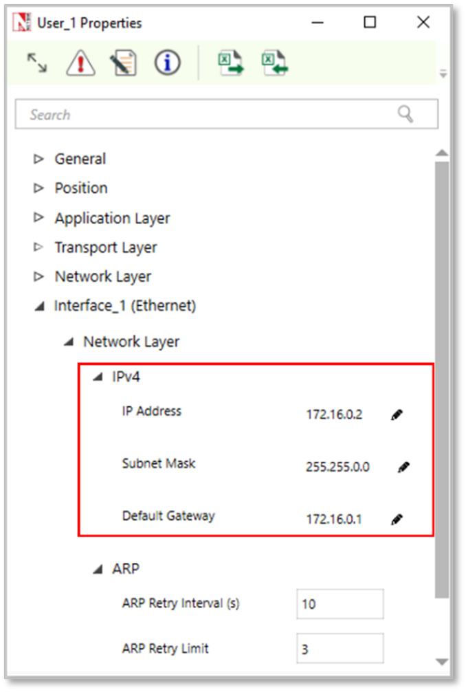
Figure-30: Configuring IP address and subnet mask in network layer of device in NetSim
Subnets using multiple switches: Here subnets have been configured using multiple switches. In the given example as shown in Figure 4 34 , we have considered 4 departments in a university campus, by configuring subnets for CS, EC, MECH, and EE. Application (traffic flow) is set for both intra and inter-subnet communication.
Department Name |
IP Address Range |
|---|---|
Computer Science (CS) |
172.16.0.1-172.16.63.254 |
Electronics and Communication (EC) |
172.16.64.1-172.16.127.254 |
Mechanical Engineering (ME) |
172.16.128.1-172.16.192.254 |
Electrical Engineering (EE) |
172.16.192.1-172.16.255.254 |
Table-21: Subnets in a university based on Table-16.

Figure-31: All the users are communicating from different subnets using a router and switch by configuring Class-B subnetting.
Firewall rules based on subnets
An important benefit of subnetting is security. Firewall/ACL rules can be configured at a subnet level. NetSim provides options for users to configure ACL/firewall rules i.e., to PERMIT or DENY traffic at a router based on (i) IP address/Network address (ii) Protocol (iii) Inbound / Outbound traffic.
Example 4: In this example, we have explained how users can set firewall rules to DENY traffic at a subnet level.
The topology considered here is the university network as shown in Figure-29.
The firewall/ACL rules are set in the Organization Router
ACL Rules:
For the CS-department Video traffic is denied
For the EC-department TCP traffic is denied
For the Mechanical department, Video Traffic is denied.
For the EE department TCP traffic is denied
These rules can be set in NetSim UI just by filling an ACL application of the router as shown below in Figure-32.

Figure-32: Setting firewall rules in the organization router
Exercises
Subnetting a Class B Network: Dividing 172.16.0.0/17 into Two Subnets
Construct the scenario as shown below and create Video and FTP application between the nodes. Using the Class B IP address range of 172.16.0.0/17, divide the network into two subnets.

Subnetting a Class C Network: Dividing 192.168.1.0 into Two Subnets
Construct the scenario as shown below and create Video and FTP application between the nodes. Using the Class C IP address range of 192.168.1.0/25, divide the network into two subnets.

Configuring the Class-A subnetting for NetSim example
Construct the following network scenario to configure Class A subnetting using the 10.0.0.0/8 IP address range. Divide the network into four subnets to optimize communication between devices, including servers and users.

Different OSPF Control Packets
There are five distinct OSPF packet types.
Type |
Description |
|---|---|
1 |
Hello |
2 |
Database Description |
3 |
Link State Request |
4 |
Link state Update |
5 |
Link State Acknowledgement |
Table-22: Different OSPF Control Packets
The Hello packets.
Hello packets are OSPF packet type 1. These packets are sent periodically on all interfaces in order to establish and maintain neighbor relationships. In addition, Hello Packets are multicast on those physical networks having a multicast or broadcast capability, enabling dynamic discovery of neighboring routers. All routers connected to a common network must agree on certain parameters (Network mask, Hello Interval and Router Dead Interval). These parameters are included in Hello packets, so that differences can inhibit the forming of neighbor relationships.
The Database Description packet
Database Description packets are OSPF packet type 2. These packets are exchanged when an adjacency is being initialized. They describe the contents of the link-state database. Multiple packets may be used to describe the database. For this purpose, a poll-response procedure is used. One of the routers is designated to be the master, the other the slave. The master sends Database Description packets (polls) which are acknowledged by Database Description packets sent by the slave (responses). The responses are linked to the polls via the packet DD sequence numbers.
The Link State Request packet
Link State Request packets are OSPF packet type 3. After exchanging Database Description packets with a neighboring router, a router may find that parts of its link-state database are out-of-date. The Link State Request packet is used to request the pieces of the neighbor’s database that are more up to date. Multiple Link State Request packets may need to be used. A router that sends a Link State Request packet has in mind the precise instance of the database pieces it is requesting. Each instance is defined by its LS sequence number, LS checksum, and LS age, although these fields are not specified in the Link State Request Packet itself. The router may receive even more recent instances in response.
The Link State Update packet
Link State Update packets are OSPF packet type 4. These packets implement the flooding of LSAs. Each Link State Update packet carries a collection of LSAs one hop further from their origin. Several LSAs may be included in a single packet. Link State Update packets are multicast on those physical networks that support multicast/broadcast. In order to make the flooding procedure reliable, flooded LSAs are acknowledged in Link State Acknowledgment packets. If retransmission of certain LSAs is necessary, the retransmitted LSAs are always sent directly to the neighbor.
The Link State Acknowledgment packet
Link State Acknowledgment Packets are OSPF packet type 5. To make the flooding of LSAs reliable, flooded LSAs are explicitly acknowledged. This acknowledgment is accomplished through the sending and receiving of Link State Acknowledgment packets. Multiple LSAs can be acknowledged in a single Link State Acknowledgment packet.
Open NetSim, Select Examples->Internetworks->Different OSPF Control Packets then click on the tile in the middle panel to load the example as shown in Figure-33.

Figure-33: List of scenarios for the example of different OSPF control packets
The following network diagram illustrates what the NetSim UI displays when you open the example configuration file for Different-OSPF-Control-Packets in NetSim as shown Figure-34.

Figure-34: Network setup for studying the different OSPF control packets.
Network Settings
Set OSPF Routing protocol under Application Layer properties of a router by clicking on the router and expanding the property panel in right.
Configure CBR application from set traffic tab from ribbon on the top. Click on created application and expand the application property panel on the right, set application Start Time(s) to 30Sec by keeping other properties as default.
Enabled Packet Trace from the configure reports tab in ribbon on the top.
Simulate for 100 sec.
Results and Discussion
The OSPF neighbors are dynamically discovered by sending Hello packets out each OSPF-enabled interface on a router. Then Database description packets are exchanged when an adjacency is being initialized. They describe the contents of the topological database. After exchanging Database Description packets with a neighboring router, a router may find that parts of its topological database are out of date. The Link State Request packet is used to request the pieces of the neighbor's database that are more up to date. The sending of Link State Request packets is the last step in bringing up an adjacency. A packet that contains fully detailed LSAs, typically sent in response to an LSR message. LSAck is sent to confirm receipt of an LSU message.
The same can be observed in Packet trace. Open packet trace from simulation results window and CONTROL PACKET TYPE/ APP NAME to OSPF HELLO, OSPF DD, OSPF LSACK, OSPF LSUPDATE and OSPF LSREQ packets as shown below Figure 4 35.
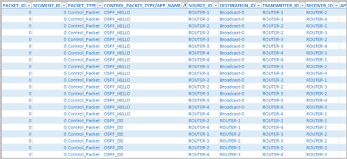

Figure-35: Different OSPF control packets in the packet Trace
Configuring Static Routing in NetSim
Static Routing
Routers forward packets using either route information from route table entries that are configured manually or the route information that is calculated using dynamic routing algorithms. Static routes, which define explicit paths between two routers, cannot be automatically updated; you must manually reconfigure static routes when network changes occur. Static routes use less bandwidth than dynamic routes. No CPU cycles are used to calculate and analyze routing updates.
Static routes are used in environments where network traffic is predictable and where the network design is simple. You should not use static routes in large, constantly changing networks because static routes cannot react to network changes. Most networks use dynamic routes to communicate between routers but might have one or two static routes configured for special cases. Static routes are also useful for specifying a gateway of last resort (a default router to which all unrouteable packets are sent).
Note that the static route configuration running with TCP protocol requires reverse route configuration.
How to Setup Static Routes
In NetSim, static routes can be configured either prior to the simulation or during the simulation.
Static route configuration prior to simulation:
Via static route GUI configuration
Via file input (Interactive-Simulation/SDN)
Static route configuration during the simulation:
Via device NetSim Console (Interactive-Simulation/ SDN)
Static route configuration via GUI
Open NetSim, Select Examples->Internetworks->Configuring Static Route then click on the tile in the middle panel to load the example as shown in Figure-36.

Figure-36: List of scenarios for the example of Configuring Static Route
The following network diagram illustrates what the NetSim UI displays when you open the example configuration file for Configuring Static Routing in NetSim as shown Figure-37.
Without Static Route

Figure-37: Network setup for studying the Configuring Static Route
Network Settings
Set grid length as 500m × 250m from grid setting property panel on the right. This needs to be done before any device is placed on the grid.
Create a scenario as shown in the above screenshot.
The default routing protocol is OSPF in application layer of routers by clicking on the router and expanding the property panel on the right.
Wired link properties are default.
Configure CBR application between wired node 6 and 7 by clicking on the set traffic tab from the ribbon at the top. Click on created application and expand the application property panel on the right and set transport protocol to UDP
Enable packet trace from configure reports tab in ribbon on the top.
Run a simulation for 10 seconds.
In packet trace, filter the CONTROL PACKET TYPE to APP1 CBR and observe the packet flow from Wired Node 6 -> Router 1-> Router 5-> Router 4-> Wired Node 7 as shown in below Figure-38.

Figure-38: Packet flows from Wired Node 6 -> Router 1 -> Router 5 -> Router 4 -> Wired Node 7
With Static Route
Static routing configuration
Open Router 1 property >Network Layer, Enable Static IP Route > Click on via GUI and set the properties as per the screenshot below and click on Add and then click on OK

Figure-39: Static IP Routing Dialogue window
This creates a text file for every router in the temp path of NetSim which is in the format below:
Router 1:
route ADD 192.169.0.0 MASK 255.255.0.0 11.0.0.2 METRIC 1 IF 1
route ADD destinationip MASK subnet_mask gateway_ip METRIC metric_value IF Interface_Id
where
route ADD: command to add the static route.
destination_ip: is the Network address for the destination network.
MASK: is the Subnet mask for the destination network.
gateway_ip: is the IP address of the next-hop router/node.
METRIC: is the value used to choose between two routes.
IF: is the Interface to which the gateway_ip is connected. The default value is 1.
Similarly Configure Static Route for all the routers as given in below Table-23.
Devices |
Network Destination |
Gateway |
Subnet Mask |
Metrics |
Interface ID |
|---|---|---|---|---|---|
Router 1 |
192.169.0.0 |
11.0.0.2 |
255.255.0.0 |
1 |
1 |
Router 2 |
192.169.0.0 |
11.0.0.10 |
255.255.0.0 |
1 |
2 |
Router 3 |
192.169.0.0 |
11.0.0.18 |
255.255.0.0 |
1 |
2 |
Router 4 |
192.169.0.0 |
192.169.0.2 |
255.255.0.0 |
1 |
3 |
Table-23: Static Route configuration for routers
After configuring the above router properties run the simulation for 10 seconds.
In packet trace, filter the CONTROL PACKET TYPE to APP1 CBR and observe the change in the packet flow from Wired Node 6 > Router 1> Router 2 > Router 3 > Router 4 > Wired Node 7 due to static route configurations as shown in Figure-40.
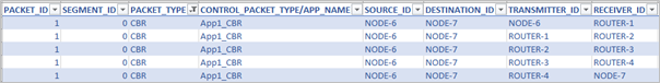
Figure-40: Packet trace shows the data flow after configuring static routes
Disabling Static Routing
If static routes were configured via GUI, it can be manually removed prior to the simulation from the Static IP Routing Dialogue or from the file input.
If static routes were configured during the run time, the entries can be deleted using the route delete command during runtime.
TCP Window Scaling
Open NetSim, Select Examples->Internetworks->TCP Window Scaling then click on the tile in the middle panel to load the example as shown in Figure-41.
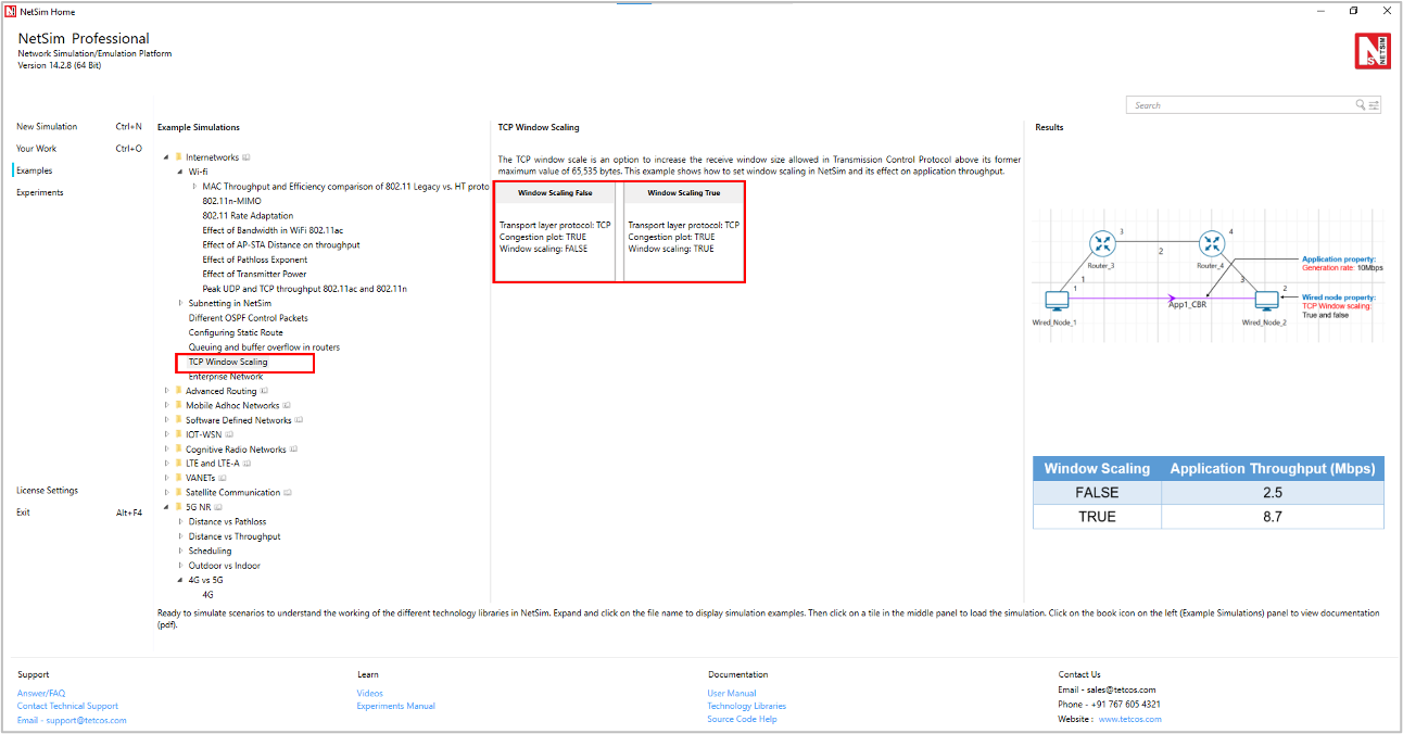
Figure-41: List of scenarios for the example of TCP Window Scaling
The following network diagram illustrates what the NetSim UI displays when you open the example configuration file for TCP Window scaling as shown Figure-42.

Figure-42: Network setup for studying the TCP Window Scaling
The TCP throughput of a link is limited by two windows: the congestion window and the receive window. The congestion window tries not to exceed the capacity of the network (congestion control); the receive window tries not to exceed the capacity of the receiver to process data (flow control).
The TCP window scale option is an option to increase the receive window size allowed in Transmission Control Protocol above its former maximum value of 65,535 bytes.
TCP window scale option is needed for efficient transfer of data when the bandwidth-delay product is greater than 64K. For instance, if a transmission line of 1.5 Mbit/second was used over a satellite link with a 513 milliseconds round trip time (RTT), the bandwidth-delay product is \(1500000 \times 0.513 = 769,500\) bits or about \(96,187\) bytes.
Using a maximum window size of 64 KB only allows the buffer to be filled to \(\frac{65535}{96187} = 68\ \%\) of the theoretical maximum speed of \(1.5\) Mbps, or \(1.02\ \)Mbps.
By using the window scale option, the receive window size may be increased up to a maximum value of \(1,073,725,440\) bytes. This is done by specifying a one-byte shift count in the header options field. The true receive window size is left shifted by the value in shift count. A maximum value of 14 may be used for the shift count value. This would allow a single TCP connection to transfer data over the example satellite link at \(1.5\) Mbps utilizing all of the available bandwidth.
Network Settings
Create the scenario as shown in the above screenshot.
To configure the properties below in the nodes, click on the node, expand the property panel on the right side, and change the properties as mentioned in the below steps.
Set TCP Window Scaling to FALSE (by default)
Enable Wireshark Capture as offline under General Properties of Wired Node 1.
Configure CBR application between two nodes by clicking on the set traffic tab from the ribbon on the top. Click on the created application and expand the application property panel on the right, packet size to 1460 and Inter arrival time to 1168 µs (Generation rate = 10Mbps).
To configure wired and wireless link properties, click on link, expand the property panel on the right and set wired link properties as shown below.
Set Bit error rate (Uplink and Downlink) to 0 in all wired links
Link1 & Link3 Propagation delay (uplink and downlink) to 5(Microsec) (by default)
Change the Link2 speed -> 10Mbps, Propagation delay (uplink and downlink) ->100000 (Microsec)
Simulate for 100sec and note down the throughput.
Now change the Window Scaling -> TRUE (for all wired nodes)
Enable Window Size vs Time plot under TCP Congestion window from the Plots tab located in the right panel.

Figure-43: Enabling TCP Congestion plot.
Simulate for 100s and note down the throughput.
Results and Discussion
Window Scaling |
Application Throughput (Mbps) |
|---|---|
FALSE |
2.5 |
TRUE |
8.7 |
Table-24: Results comparison for with/without Window Scaling
Throughput calculation (Without Window Scaling)
Theoretical Throughput = Window size / Round trip time = \(\frac{65525*8\ Bytes}{200ms}\ \) = \(\ 2.62\ Mbps\ \)
Go to the simulation result window -> plots -> TCP Congestion Window Plot Figure-45/Figure-46.

Figure-44: Open TCP Congestion Window plot from the result dashboard.

Figure-45: TCP Congestion Window Plot for wired node 2.
In Window Scaling False, the Application Throughput is 2.5 Mbps less than the theoretical throughput since it initially takes some time for the window to reach 65535 B.

Figure-46: TCP Congestion Window Plot for wired node 2.
In Window Scaling TRUE, From the above screenshot, users can notice that the window size grows up to 560192Bytes because of Window Scaling. This leads to a higher Application throughput compared to the case without window scaling.
We have enabled Wireshark Capture in the Wired Node 1. The PCAP file is generated silently at the end of the simulation. Double click on WIRED NODE1_1.pcap file available in the result window under packet captures, In Wireshark, the window scaling graph can be obtained as follows. Select any data packet with a left click, then, go to Statistics > TCP Stream Graphs > Window Scaling > Select Switch Direction.

Figure-47: Wireshark Window when Window Scaling is TRUE.
An enterprise network comprising of different subnets and running various applications
We consider a simple enterprise network, comprising of two branches, headquarters and a data center. Branches and headquarters are connected to the data center over the public cloud. Branch 1 has 10 systems, branch 2 has 10 systems, HQ has 5 systems, and they connect to a data center which houses a DB server, an email server, and an FTP server.
Open NetSim, Select Examples->Internetworks->Enterprise Network then click on the tile in the middle panel to load the example as shown in Figure-48.

Figure-48: List of scenarios for the example of enterprise networks
The following network diagram illustrates what the NetSim UI displays when you open the example configuration file for Enterprise Network in NetSim as shown in Figure-49.

Figure 4 49: Network setup for studying the enterprise network. Labelling (Branch-1, Branch-2, HQ, Data center) has been added to the screen shot. Links 29, 30 and the WAN Router can be thought of as the internet cloud over which traffic flows to reach the data center.
Network Settings
Enterprise Network I
Link rate for the outbound link i.e., link 28 from Branch 1 is set to 2 Mbps. Link properties can be set by clicking on the click, expanding the link properties panel on the right.

Figure-50: Setting link speed for outbound link (link 28)
Configure one FTP application from 7 to the file server 39, a DB application from 6 to the Database server 41, and eight email applications running between 8,9,10, 23, 25, 24, 26, 27 and the Email server 40. Refer to 3.9.3.2 section in user manual to configure multiple applications using rapid configurator.
Run the simulation for 100 s.
Enterprise Network II
In this sample, we add more nodes via the switch and configured 3 FTP applications from systems 11, 12, 13 i.e. Wired node 43, 44 and 45 to FTP server 39 as shown in Figure-51 By keeping the Link rate for the outbound link (link 28) as 2 Mbps.

Figure-51: Configuring FTP applications from systems 43,44,45 to FTP server 39
Simulate for 100 seconds.
Enterprise Network III
In this sample, we change the outbound link speed i.e., Link 28 to 4 Mbps and simulate for 100 seconds.
Enterprise Network IV
In this sample, we change the outbound link speed i.e., Link 28 to 2Mbps and configure Voice applications from 14, 15, 43, 44 and 45 to Head office 10 as shown in Figure-52.

Figure-52: Configuring voice applications from 14, 15, 43, 44 and 45 to Head office 10.
Also, Scheduling type is set to Priority under Network Layer Properties of Router 38 Interface WAN properties as shown below Figure-53.
Figure-53: WAN Interface – Network layer properties window
Simulate for 100 seconds.
Results and Discussion
Enterprise Network I: In the simulation results window, observe the application metrics and calculate the average delay for email application as shown below. For earlier delay calculations, the user can also export the results by clicking on the export results option present in the simulation results window

Figure-54: Application metrics table for Enterprise Network I.
The average delay experienced by the e-mail applications is 2.69 s.
Enterprise Network II: In this sample, the average delay for email applications increases to 15.79 s due to the impact of additional load on the network.
Enterprise Network III: In this sample, the average delay for e-mail applications has dropped down to 0.68 s due to the increased link speed.
Enterprise Network IV: In this sample, the average delay for the e-mail application has increased to 5.73 s since voice has a higher priority over data. Since priority scheduling is implemented in the routers, they first serve the voice packets in the queue and only then serve the email packets.
Design of a nationwide university network to analyze capacity, latency, and link failures
Introduction
SWITCHlan is the national research and education network in Switzerland. It is operated by SWITCH, the Swiss National Research and Education Network organization. This network connects Swiss universities, research institutions, and other educational organizations, providing them with high-speed and reliable network connectivity. It allows Swiss institutions to benefit from global connectivity and participate in international research collaborations.

Figure-55: The network connection between universities of different cities in Switzerland
NetSim allows you to model and simulate complex networks, including LANs and WANs, using different types of network devices. By abstracting SWITCHlan with routers and WAN links in NetSim, you can simulate various traffic loads, test different configurations, and evaluate the performance of the network under different conditions.
In this study, we simulate SWITCHlan by modeling six universities located in Lausanne, Zurich, Basel, Bern, Luzern, and Fribourg. Each university is represented by a router and a server. WAN links connect these routers, simulating the network topology of SWITCHlan.

Figure-56: Network Scenario in NetSim representing the different cities.
Open NetSim, Select Examples -> Internetworks -> Design of a nationwide university network to analyze capacity, latency, and link failures then click on the tile in the middle panel to load the example shown in below

Figure-57: List of scenarios for the example of design of nationwide university network to analyze capacity, latency, and link failures
Network Settings
Drop 6 routers and wired node (server) in NetSim design window as shown in Figure-58. This represents six different countries.
Connect the devices as shown in scenario and set the link capacity for all wired links to 10 Mbps.
Application layer routing protocol is set to OSPF in router.
Configure the custom application from each city to every other city (30 flows in total) to enable data transfer. Refer to Table-25 for application properties.
Enable Packet Trace from the configure reports tab in ribbon on the top.
Enable latency and throughput plots by clicking on the Plots/Logs tab in the right panel.
Simulate the scenario for 50 seconds.

Figure-58: This figure shows the traffic configuration between all cites. Since there are 6 cities, there is a total of 6*5 = 30 traffic flows.
Simulation cases and Application settings
Case 1: Regular Operation (Traffic Rate 1.9 Mbps)
A traffic rate of 1.9 Mbps is chosen because there are five flows passing through each bottleneck link (connecting a router to a server) in one direction. These five flows represent the traffic coming from and going to the other five cities. Consequently, the bottleneck flow rate is approximately 2 Mbps (10 Mbps/5). To avoid saturation, the traffic rate is set slightly below this capacity at 1.9 Mbps per flow. The parameter configuration is as follows:
Parameter |
Value |
|---|---|
Application Parameters |
|
Application type |
Custom |
Transport Protocol |
UDP |
Traffic Configuration |
UL & DL between all cities. |
Packet Size – Value |
1460 bytes |
Packet Size – Distribution |
Constant |
Inter Arrival Time – Mean |
6147\(\ \mu s\) |
Inter Arrival Time – Distribution |
Exponential |
Table-25: Application settings for case1
Case 2: Increased Traffic Load (Traffic Rate 1.95 Mbps)
Parameter |
Value |
|---|---|
Application Parameters |
|
Application type |
Custom |
Transport Protocol |
UDP |
Traffic Configuration |
UL & DL between all cities. |
Packet Size – Value |
1460 byte |
Packet Size – Distribution |
Constant |
Inter Arrival Time – Mean |
5989\(\mu s\) |
Inter Arrival Time – Distribution |
Exponential |
Table-26: Application settings case2
Case 3: Link Failure (Basel-Zurich Link)
In this case, the traffic configuration is similar to Case 1 (1.9 Mbps). However, here we study the impact of a link failure by failing the link between Basel and Zurich at 10 seconds in the Link 4 properties, as shown below.

Figure-59: Configuring the link failure for link 4(between Basel and Zurich)
Parameter |
Value |
|---|---|
Application Parameters |
|
Application type |
Custom |
Transport Protocol |
UDP |
Traffic Configuration |
UL & DL between all cities. |
Packet Size – Value |
1460 byte |
Packet Size – Distribution |
Constant |
Inter Arrival Time – Mean |
6147\(\ \mu s\) |
Inter Arrival Time – Distribution |
Exponential |
Table-27: Application settings case3
Traffic is rerouted via alternate paths using OSPF protocol
Results and Observations
Case 1: Regular Operation
In the application metrics, we observe that the total packets generated are 7,978, packets received are 7,922, and errored packets are 56.

Figure-60: Results obtained for case1 in Application Metrics
The mean generation rate is 1.90 Mbps, and the obtained throughput is 1.85 Mbps. The small difference is due to the errored packets
Now click on plots from Left hand side of result dashboard to access throughput and latency plots

Figure-61: Accessing Throughput vs Time and Latency vs Time plots
To plot an application's throughput or Latency, select the Application Name from the dropdown, and click on Plot.

Figure-62: Plotting Throughput vs Time
Throughput plots: (Lausanne to Zurich & Zurich to Lausanne)
The following plots shows the throughput vs time for:

Figure-63: NetSim plot of throughput vs. time for traffic flowing from Lausanne to Zurich and Zurich to Lausanne
The spread occurs because we are generating a variable bit rate, not a constant one, with a mean of 1.9 Mbps. This is achieved using an exponential random variable for inter-arrival time to simulate real-world traffic flow
Latency plots: (Lausanne to Zurich & Zurich to Lausanne)
The following plots show the Latency vs. Time for traffic between Lausanne and Zurich Servers

Figure-64: NetSim plot of Latency vs. time for traffic flowing from Lausanne to Zurich and Zurich to Lausanne
We see that the average latency is not continuously increasing, but only varies around a mean. From this, we can infer that the network is able to fully handle the traffic flows between these two end points.
OSPF convergence time: We define the time at which the first data packet is forwarded by the Router as the convergence time. From the packet trace, we see that in this example, OSPF tables have converged at time ~1217 µs or 1.2 ms (highlighted in orange). The 3 entries seen in the packet trace at 1217 µs are transmissions starting at 3 routers after table convergence.

Figure-65: OSPF Convergence time shown in packet trace
Case 2: Increased Traffic Load
We observe application throughput is less than the generation rate of 1.95. However, we cannot immediately say if the network can or cannot handle this traffic load of 1.95 Mbps. To correctly estimate we need to observe how latency varies with time

Figure-66: Results obtained for case2 in Application Metrics
Throughput plots: (Lausanne to Zurich & Zurich to Lausanne)
The following plots shows the throughput vs time for:

Figure-67: NetSim plot of throughput vs. time for traffic flowing from Lausanne to Zurich and Zurich to Lausanne
Latency plots: (Lausanne to Zurich & Zurich to Lausanne)
The following plots show Latency vs. Time for traffic between Lausanne and Zurich Servers

Figure-68: NetSim plot of Latency vs. time for traffic flowing from Lausanne to Zurich and Zurich to Lausanne
We see latency increasing with time. This is a sign of queuing and an indication that the network is unable to handle the traffic load of 1.95 Mbps. Saturation occurs somewhere between 1.90 to 1.95 Mbps.
Case 3: Link Failure Analysis
Next, we study the impact of link failure. To do so, we fail the Basel – Zurich link at t = 10s by setting downtime to 10s in link 4 properties.
Throughput plots: (Lausanne to Zurich & Zurich to Lausanne)

Figure-69: NetSim plot of throughput vs. time for traffic flowing from Lausanne to Zurich and Zurich to Lausanne
Latency plots: (Lausanne to Zurich & Zurich to Lausanne)

Figure-70: NetSim plot of Latency vs. time for traffic flowing from Lausanne to Zurich and Zurich to Lausanne
Latency starts spiking up at the 10th second when the Basel – Zurich link fails.
Pre-failure average delay is ~51 ms
Post-failure average delay: 5025 ms (5 seconds)
Basel – Zurich Link
Application Throughput (Mbps) and Latency plots

Figure-71: NetSim plot of Throughput & Latency vs. time for traffic flowing from Basel to Zurich.
After the direct Basel-Zurich link fails:
Pre-failure average delay: \(\sim 61\) ms
Post-failure average delay: \(\sim 2373\) ms (2.4 seconds)
The new route taken by the packets, i.e., Basel > Bern > Luzern > Zurich and can be observed from the packet trace.
OSPF convergence time
Initially, routes converge at time at \(\sim 1217\) µs or 1.22 ms
Before link failure, data flows using link 4 are Basel-Luzern, Basel-Zurich, Bern-Zurich, Fribourg-Zurich and Lausanne-Zurich
Transmissions in Link 4 get disrupted at 10 sec
It then takes approximately an average of 30 ms for OSPF to converge
During link failure, packet buffer at the router since packets can no longer be sent over the failed link
Once OSPF converges packets queued in the router buffer - along with newly arriving packets - start getting transmitted in the new route
For example, in the Bern-Zurich traffic flow the new route is obtained and data transmissions start at 10.030 s.
In packet trace in CONTROL_PACKET_TYPE/APP_NAME filter BERN_TO_ZURICH and BASEL_TO_ZURICH and OSPF_LSUPDATE
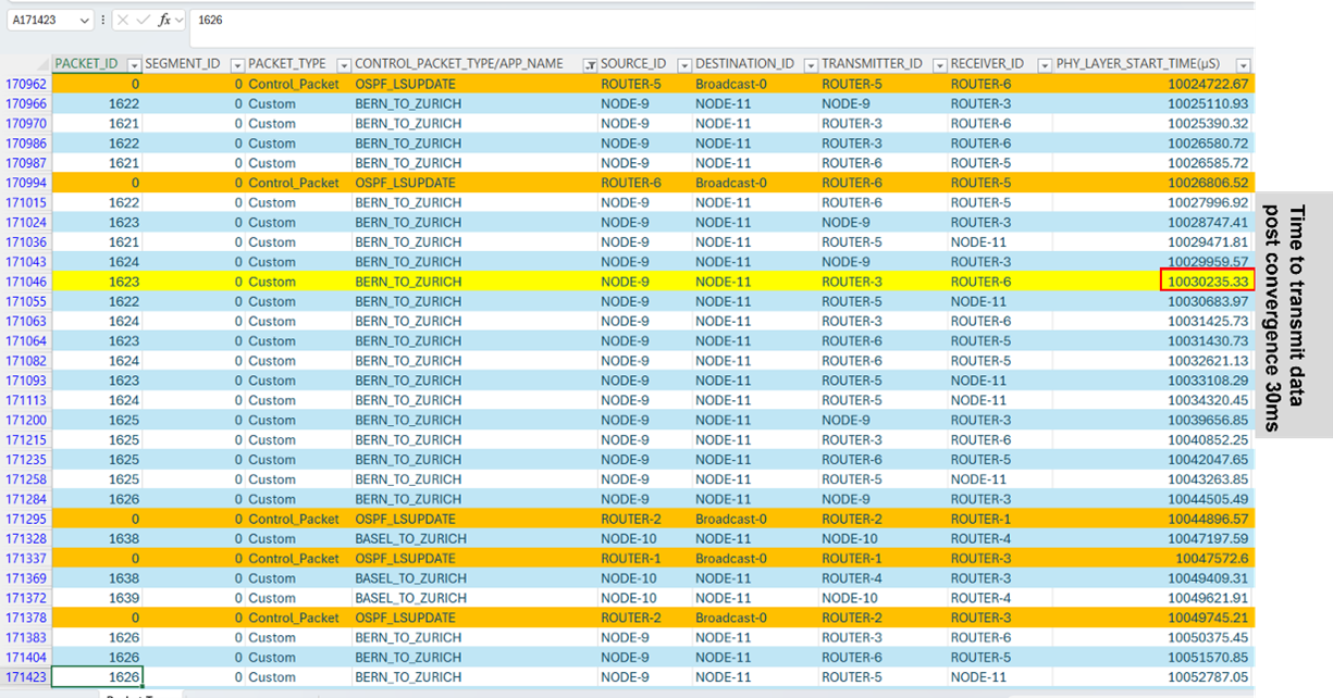
Figure-72: OSPF Convergence time after link failure is shown in packet trace