Featured Examples
Throughput and delay variation with distance
Open NetSim and Select Examples \(\rightarrow\) Underwater Acoustic Network \(\rightarrow\) Throughput and delay variation with distance and then click on the tile in the middle panel to load the example as Figure 1.
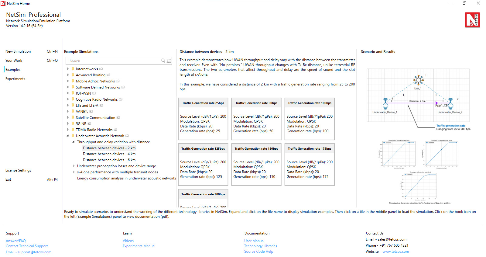
In this example, we understand how UWAN throughput and delay varies as the distance between 1 transmitter and 1 receiver is varied. Even with no pathloss the throughput in UWAN varies with Tx-Rx distance which is not the case in terrestrial RF based transmissions. The two parameters that affect throughput and delay are the speed of sound and the slot length of s-Aloha. The speed of sound in water is given by the formula
\[\begin{multline} {c}_{sound}=1449.05+45.7t-5.21\times {t}^{2}+ 0.23\times {t}^{3} \\ +\left( 1.333-0.126t+0.009\times {t}^{2}\right)\left(S-35\right)+16.3\times z+0.18\times {z}^{2} \end{multline}\]
where \(t\) is one-tenth of the temperature of the water in degrees Celsius, \(z\) is the depth in km and \(S\) is the salinity of the water in ppt. Then using \(t=\frac{25}{10}=2.5,\) \(z=50\), and \(S=35\) - where t is one-tenth of the temperature of the water in degrees Celsius, z is the depth in meters and S is the salinity of the water - we get \({c}_{sound}=2799.33\ m/s\). When the transmitter receiver distance is \(d=2km\), the propagation delay, \(\Delta =\frac{2\times 10^{3}}{2799.33}= 714{,}456.4\ \mu s\)
Next, as explained in section 3.2.2, we consider ideal slot lengths for different transmitter receiver distances. In the case when \({d}_{Rx}^{Tx}=2\ km\) the slot length turns out as
\[\begin{equation} {L}_{Slot}= {T}_{tx}+\Delta =16{,}800+714{,}456.4=731{,}256.4\ \mu s=0.73 \end{equation}\]
Table 5 shows the ideal slot length settings for \({d}_{Rx}^{Tx}=4\ km\) and \({d}_{Rx}^{Tx}=6\ km.\)
Network setup:
The following network diagram illustrates what the NetSim UI displays when you open the example configuration file.

In case #1, distance between the underwater devices is set to be 2km. In case #2 the distance is 4km, while in case #3 it is set to 6 km
Click on link, expand the property panel on the right and set the Channel characteristics as No pathloss.
Device Configuration:
| Device \(>\) Interface (ACOUSTIC) \(>\) Datalink Layer | |
|---|---|
| Slot Length (\(\mu\)s) | 731257 for 2 km |
| Device \(>\) Interface (ACOUSTIC) \(>\) Physical Layer | |
| Source Level () | 200 |
| Modulation | QPSK |
| Data Rate (kbps) | 20 |
Application Configuration:
We run simulations for different traffic generation rates. The generation rate depends on the inter arrival time – a GUI input in NetSim – in the following way
\[\begin{equation} \text{Generation Rate (Mbps)}=\frac{\text{Packet Size (Bytes)} \times 8}{\text{Interarrival Time ($\mu$s)}} \end{equation}\]
| Application Properties | |
|---|---|
| Application Method | App1 CBR |
| Source ID | 1 |
| Destination ID | 2 |
| Packet Size (Bytes) | 14 |
| Inter arrival Time (\(\mu\)s) | Generation rate (bps) | |
|---|---|---|
| Case-1 | ||
| 4480000 | 25 | |
| 2240000 | 50 | |
| 1120000 | 100 | |
| 896000 | 125 | |
| 746666.6666 | 150 | |
| 640000 | 175 | |
| 560000 | 200 | |
| Case-2 | ||
| 5600000 | 20 | |
| 2800000 | 40 | |
| 1866666.6666 | 60 | |
| 1400000 | 80 | |
| 1120000 | 100 | |
| Case-3 | ||
| 5600000 | 20 | |
| 3733333.333 | 30 | |
| 2800000 | 40 | |
| 2240000 | 50 | |
| 1866666.6666 | 60 | |
| 1600000 | 70 | |
Enable packet trace and Acoustic Measurements Log under Configure report tab as shown below

Run the Simulation for 100 sec.
Theoretical Predictions
The predicted propagation delay when the speed of sound \({c}_{sound}=2799.33\ m/s\) is
| Distance between devices | Propagation delay (\(\mu\)s) |
|---|---|
| 2km | 714456.4 |
| 4km | 1428912.7 |
| 6km | 2143369.1 |
Transmission delay and Saturation Throughput
Considering a slot length of \(731{,}257\ \mu s\), we see that one packet exactly fits one slot and hence the predicted saturation throughput would be
\[\begin{equation} {\theta}_{sat}^{2km}=\frac{{(L}_{pkt}\times 8)}{{L}_{slot}}=\frac{\left(14\times 8\right)}{731256.4\times {10}^{-6}}=153\ bps \end{equation}\]
Proceeding similarly for 4 km and 6 km, the predictions for saturation throughput are
| Distance between devices | Slot Length (\(\mu\)s) | Saturation Throughput (bps) |
|---|---|---|
| 2 km | 731257 | 153 |
| 4 km | 1445713 | 77 |
| 6 km | 2160170 | 52 |
Simulation results
We calculate queuing delay, transmission delay, and propagation delay from the packet trace. The steps are:
Open Packet Trace file using the Packet Trace option available in the Simulation Results window under traces.
The difference between the PHY LAYER ARRIVAL TIME(US) and the MAC LAYER ARRIVAL TIME(US) will give us the delay of a packet. (Refer Figure 3)
\[\begin{multline} \text{Queuing Delay}\ (\mu s)=\text{PHYSICAL LAYER ARRIVAL TIME}(\mu s)\\ -\text{MAC LAYER ARRIVAL TIME}\ (\mu s) \end{multline}\]

Now, calculate the mean queuing delay by taking the average of the queueing delays of all the packets. This is nothing but the column average. (Refer Figure 3)
Similarly, users can get the Mean Transmission Delay and Mean Propagation Delay from the packet trace using the formulas
\[\begin{multline} \text{Transmission Delay}\ (\mu s)=\text{PHY LAYER START TIME}(\mu s)\\ -\text{PHY LAYER ARRIVAL TIME}(\mu s) \end{multline}\]
\[\begin{multline} \text{Propagation Delay}\ (\mu s)=\text{PHY LAYER END TIME}(\mu s)\\ -\text{PHY LAYER START TIME}(\mu s) \end{multline}\]
| Case | Gen. Rate (bps) | Thruput (bps) | Delay (\(\mu\)s) | Mean Prop. Delay (\(\mu\)s) | Mean Tx Delay (\(\mu\)s) | Mean Queue Delay (\(\mu\)s) |
|---|---|---|---|---|---|---|
| Case #1: Distance between underwater devices is 2km | ||||||
| 25 | 26 | 1113144.78 | 714456.35 | 16800 | 381888.43 | |
| 50 | 50 | 1111731.73 | 714456.35 | 16800 | 380475.37 | |
| 100 | 100 | 1094568.64 | 714456.35 | 16800 | 363312.29 | |
| 125 | 124 | 1091089.64 | 714456.35 | 16800 | 359833.28 | |
| 150 | 149 | 1116252.45 | 714456.35 | 16800 | 384996.10 | |
| 175 | 152 | 6891103.855 | 714456.35 | 16800 | 6159847.5 | |
| 200 | 152 | 12291103.8 | 714456.35 | 16800 | 11559847.5 | |
| Case #2: Distance between underwater devices is 4km | ||||||
| 20 | 20 | 2036146.04 | 1428912.7 | 16800 | 590433.33 | |
| 40 | 40 | 2081859.04 | 1428912.7 | 16800 | 636146.33 | |
| 60 | 59 | 2148454.18 | 1428912.7 | 16800 | 702741.47 | |
| 80 | 77 | 2999954.70 | 1428912.7 | 16800 | 1554242 | |
| 100 | 77 | 12519954.7 | 1428912.7 | 16800 | 11074242 | |
| Case #3: Distance between underwater devices is 6km | ||||||
| 20 | 20 | 3163994.06 | 2143369.06 | 16800 | 1003825 | |
| 30 | 30 | 3230739.43 | 2143369.06 | 16800 | 1070570.37 | |
| 40 | 39 | 3194853.63 | 2143369.06 | 16800 | 1034684.57 | |
| 50 | 49 | 3340415.65 | 2143369.06 | 16800 | 1180246.5 | |
| 60 | 52 | 8763994.06 | 2143369.06 | 16800 | 6603825 | |
| 70 | 52 | 14763994.0 | 2143369.06 | 16800 | 12603825 | |

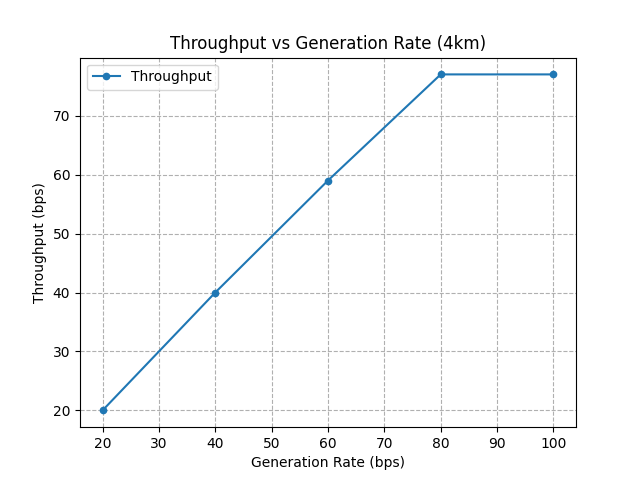
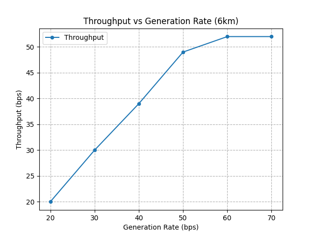
From Table 6, we see that the propagation delays from simulation match predictions in Table 4. Then we observe that saturation throughput (the Y axis value once the curve flattens) matches prediction.
| Distance between devices | Saturation Throughput Predicted (bps) | Saturation Throughput Simulation (bps) |
|---|---|---|
| 2 km | 153 | 152 |
| 4 km | 77 | 77 |
| 6 km | 52 | 52 |
Underwater propagation losses and device range
Open NetSim and Select Examples \(\rightarrow\) Underwater Acoustic Network \(\rightarrow\) Underwater propagation losses and device range and then click on the tile in the middle panel to load the example as Figure 4.

In this example, we understand the Thorp propagation model, the sources of underwater noise, the passive sonar equation and how device range can be estimated based on received SNR. Refer to section 3.1 for the underlying theory on signal level, transmission losses, and the passive sonar equation.
In the NetSim GUI, we provide 3 samples per modulation scheme, totaling 18 samples for the 6 modulation techniques. The complete set of configuration files (scenario, settings and other related files) comprising of 621 samples, is available at https://github.com/NetSim-TETCOS/UWAN_Examples_v14.4/archive/refs/heads/main.zip.
Click on the link given and download UWAN Experiments
Extract the zip folder. The extracted project folder consists of Underwater propagation losses and device range example files.
How to import the workspace is explained in section 4.9.2 in NetSim User Manual.
Network setup
The following network diagram illustrates what the NetSim UI displays when you open the example configuration file.
Click on link, expand the right-side property panel and set the Channel characteristics as Pathloss Only.
Click on Underwater Device 1, expand the right-side property panel change the following parameters,
| Device Properties \(>\) Physical Layer | |
|---|---|
| Source Level () | 190.8, 187.78, 183.81 |
| Data Rate (kbps) | 20 |
| Modulation Technique | QPSK, BPSK, FSK, 16QAM, 64QAM, 256QAM |
Configure a CBR Application from Source ID as 1 and Destination ID as 2 from set traffic window present in the ribbon at the top with Default Properties.
Enable packet trace and Acoustic Measurements Log under Configure report tab as shown in Figure 2.
Run the Simulation for 1000 sec.
Analytical computations
In the Thorp model, the \(dB/km\) attenuation is given by
\[\begin{equation} 10\log_{10}(\alpha \left(f\right))=\begin{cases} 0.11\times \dfrac{f^{2}}{1+f^{2}}+ 44\times \dfrac{f^{2}}{4100+f^{2}}+2.75\times 10^{-4}\times f^{2}+0.003 & f\geq 0.4\ \text{kHz} \\[10pt] 0.002+0.11\times \dfrac{f^{2}}{1+f^{2}}+0.011\times f^{2} & f<0.4\ \text{kHz} \end{cases} \end{equation}\]
For this example, substituting \(f=20,\) we get \(10\log_{10}(\alpha \left(f\right))=4.133\ dB/km\), we see that the total pathloss is
\[\begin{equation} 10 \log A\left(d, f\right)= k\times 10 \log ({d}_{m}) +{d}_{km}\times 10 \log \alpha (f) \end{equation}\]
Using input parameters \(K\ (\text{spread coefficient})=2, f=20\ kHz\) and distance between the source and destination, \(d=18\ km\), and we get the total transmission loss, \(TL,\) as
\[\begin{equation} TL= 10 \log A\left(d, f\right)=159.51\ dB \end{equation}\]
Next, we turn to noise level \(NL.\) The turbulence, shipping, wind, and thermal, noise level in dB is given by
\[\begin{align} 10 \log{N}_{t}\left(f\right) &= 17 - 30\log( f) \\ 10 \log{N}_{s}\left(f\right) &= 40 + 20\times \left(s - 0.5\right)+ 26 \log f -60\times \log(f + 0.03) \\ 10 \log{N}_{w}\left(f\right) &= 50 + 7.5\times \sqrt{w} + 20 \log f-40 \log\left(f + 0.4\right) \\ 10 \log{N}_{th}(f) &= -15 + 20 \log f \end{align}\]
Substituting \(f=20\ kHz,\) shipping factor \(s=0.5,\) surface windspeed \(w=0\ m/s,\) we get \({N}_{t}=-22.03\ dB\), \({N}_{s}=-4.27\ dB,\) \({N}_{w}=23.63\ dB\), and \({N}_{th}=11.02\ dB\). As explained in section 3.1.4 we see that wind noise has the most impact. After adding these noises in the linear scale and then converting back to \(dB\), Total noise, \({N}_{Total}^{dB}=23.87\). From the passive sonar equation
\[\begin{equation} SNR=SL-TL-(NL-DI) \end{equation}\]
Substituting we get
\[\begin{equation} SNR=190.80-159.51-\left(23.87-0\right)=1.41\ dB \end{equation}\]
Results: Packet Error Rate vs Distance
For the above SNR, we plot PER vs. distance for different modulation schemes given default packet size of 14B.
\[\begin{equation} PER=\frac{\text{No. of errored packets}}{(\text{No. of errored packets}+\text{No. of received packets})} \end{equation}\]
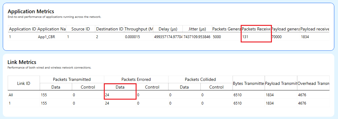
No. of errored packets can be obtained from link metrics and No. of received packets can be obtained from application metrics of the results dashboard as shown in the image below.
| Distance (m) | Source Level (dB/\(\mu\)Pa) | Modulation | Pkts Received | Pkts Errored | PER |
|---|---|---|---|---|---|
| 18000 | 183.81 | FSK | 0 | 19 | 1 |
| 18000 | 183.81 | BPSK | 0 | 19 | 1 |
| 18000 | 183.81 | QPSK | 0 | 19 | 1 |
| 18000 | 187.78 | FSK | 0 | 19 | 1 |
| 18000 | 187.78 | BPSK | 0 | 19 | 1 |
| 18000 | 187.78 | QPSK | 0 | 19 | 1 |
| 18000 | 190.8 | FSK | 0 | 19 | 1 |
| 18000 | 190.8 | BPSK | 131 | 24 | 0.154839 |
| 18000 | 190.8 | QPSK | 0 | 19 | 1 |
| 23000 | 183.81 | 16QAM | 119 | 2 | 0.016529 |
| 23000 | 183.81 | 64QAM | 32 | 41 | 0.561644 |
| 23000 | 183.81 | 256QAM | 0 | 13 | 1 |
| 23000 | 187.78 | 16QAM | 121 | 0 | 0 |
| 23000 | 187.78 | 64QAM | 119 | 2 | 0.016529 |
| 23000 | 187.78 | 256QAM | 7 | 22 | 0.758621 |
| 23000 | 190.8 | 16QAM | 121 | 0 | 0 |
| 23000 | 190.8 | 64QAM | 121 | 0 | 0 |
| 23000 | 190.8 | 256QAM | 113 | 8 | 0.066116 |

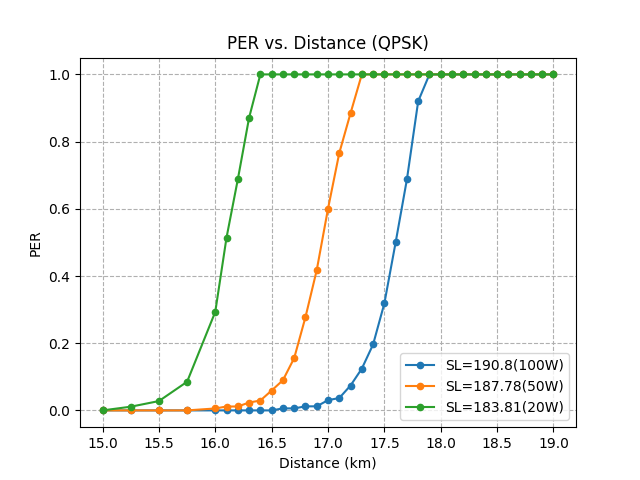

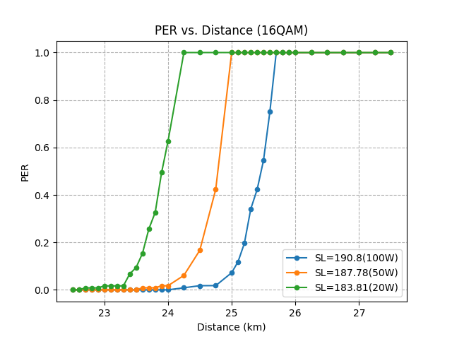
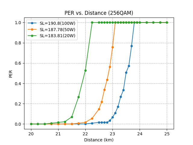

Generally, range is defined as the Tx-Rx distance at which the PER is 10%. From these plots we can determine a device’s range. In summary, we see how the device range is dependent on Source Level, Noise, MCS and packet size.
s-Aloha performance with multiple transmit nodes
Open NetSim and Select Examples \(\rightarrow\) Underwater Acoustic Network \(\rightarrow\) s-Aloha performance with multiple transmit nodes and then click on the tile in the middle panel to load the example as Figure 5.

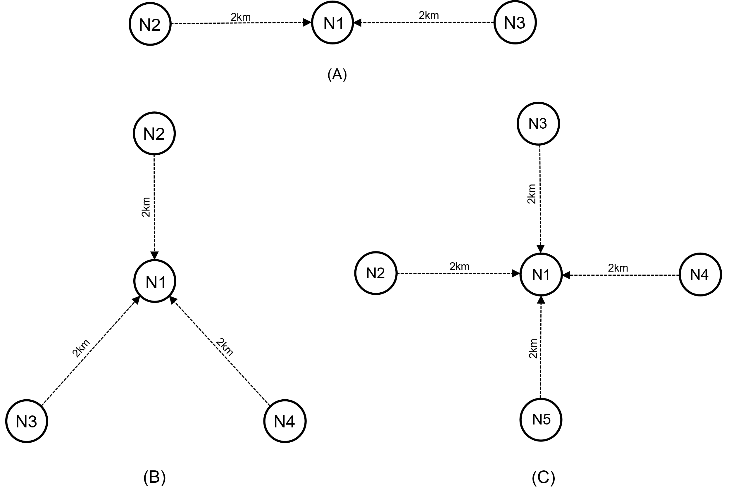
Network setup
We consider three scenarios as shown in the figure below, with 2, 3 and 4 transmitting nodes.
Properties
Then we set the UWAN device properties as shown below
| Device Properties | |
|---|---|
| Device \(>\) Interface (ACOUSTIC) \(>\) Datalink Layer | |
| Retry Limit | 0, 4, 6 |
| Slot Length (\(\mu\)s) | 741257 |
| Device \(>\) Interface (ACOUSTIC) \(>\) Physical Layer | |
| Source Level () | 190.8 |
| Modulation | QPSK |
| Data Rate (kbps) | 20 |
Here, we set the Slot Time as 741257 \(\mu s\), which is the ideal value of 731257 \(\mu s\) plus a guard interval of 10,000 \(\mu s\)
Configure a CBR Application from the source nodes (2, 3, 4 and 5 per the cases) to the destination (Node 1) with a packet size of 14 bytes and Inter arrival time as 560000 \(\mu s\) from set traffic window present in the ribbon at the top.
Enable packet trace and Acoustic Measurements Log under Configure report tab as shown in Figure 2.
Run the Simulation for 10000 sec.
Results
We observe throughputs from network metrics and packets transmitted and packets collided from the Link Metrics. We compute collision probability as \({P}_{c}=\frac{\text{Collision Count}}{\text{Packet Transmitted}}\) and tabulate the results in the different cases.
| Case #1: Two transmitting nodes | ||||||
|---|---|---|---|---|---|---|
| Retry Limit | Thru. N1 (bps) | Thru. N2 (bps) | Agg. Thru. (bps) | Collision Count | Pkt Tx | \(P_c\) |
| 0 | 0 | 0 | 0 | 26980 | 26980 | 1 |
| 4 | 51 | 55 | 106 | 7104 | 16624 | 0.427 |
| 6 | 65 | 71 | 136 | 2548 | 14647 | 0.173 |
| Case #2: Three transmitting nodes | |||||||
|---|---|---|---|---|---|---|---|
| Retry Limit | Thru. N1 (bps) | Thru. N2 (bps) | Thru. N3 (bps) | Agg. Thru. (bps) | Collision Count | Pkt Tx | \(P_c\) |
| 0 | 0 | 0 | 0 | 0 | 40470 | 40470 | 1 |
| 4 | 26 | 26 | 27 | 79 | 12234 | 19348 | 0.632 |
| 6 | 43 | 41 | 37 | 121 | 4969 | 15726 | 0.316 |
| Case #3: Four transmitting nodes | ||||||||
|---|---|---|---|---|---|---|---|---|
| Retry Limit | Throughput N1 (bps) | Throughput N2 (bps) | Throughput N3 (bps) | Throughput N4 (bps) | Aggregate Throughput (bps) | Collision Count | Packet Transmitted | \(P_c\) |
| 0 | 0 | 0 | 0 | 0 | 0 | 53960 | 53960 | 1 |
| 4 | 15 | 15 | 14 | 16 | 60 | 16942 | 22293 | 0.75 |
| 6 | 28 | 27 | 26 | 26 | 107 | 7202 | 16756 | 0.42 |
We carry out simulations with different settings of Retry Count. The final results are plotted below. When Retry count is set to zero, all packets collide even when just two nodes are transmitting. With retry count set to 0, the node attempts a packet transmission. If it fails, there is no retry and the packet is dropped. Recall, that in s-Aloha the transmitter does not back off before the first transmission attempt for a packet. With backlogged queues, the two transmitting nodes keep attempting at each slot. This leads to continuous collisions.
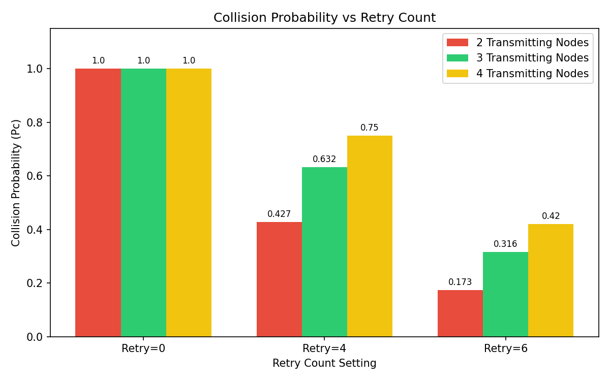
When the retry count is set to 4 (or 6) a transmitting node back off per the exponential backoff algorithm, before every retransmission. The back off algorithm is explained in section 3.2.3. Hence there is an element of randomness in packet transmissions at each slot. Nodes may or may not transmit. The probability of transmission at a particular slot reduces as the Retry Count is increased. Hence, we see lower collision probabilities for Retry count of 6.
Energy consumption analysis in underwater acoustic networks under varying traffic loads
Introduction
Efficient energy usage is important for underwater devices because the underwater environment imposes constraints on recharging options. Optimizing energy consumption is essential to ensure the longevity of the network.
Consider a practical underwater acoustic network comprising sensor nodes deployed in the ocean, which collect data and relay it to a master node. This master node aggregates the data, transfers it to a shore-based control center, and controls the sensor nodes. The network traffic consists of packetized data delivery from the sensor nodes to the master node.
In our project, we model such a network in NetSim. The setup includes master and sensor nodes distributed across 16 underwater devices, organized into three clusters (A, B, and C). Each cluster contains sensor nodes responsible for data collection and transmission, with the master node managing data aggregation. The scenario is based on [9].
We analyse the energy consumption patterns of the sensors and the master node under different traffic loads.
Open NetSim and Select Examples \(\rightarrow\) Underwater Acoustic Network \(\rightarrow\) Energy consumption analysis in underwater acoustic networks under varying traffic loads and then click on the tile in the middle panel to load the example as shown in figure.

Network setup
The scenario comprises of 16 underwater devices, organized into three clusters (A, B, and C) and a master node.
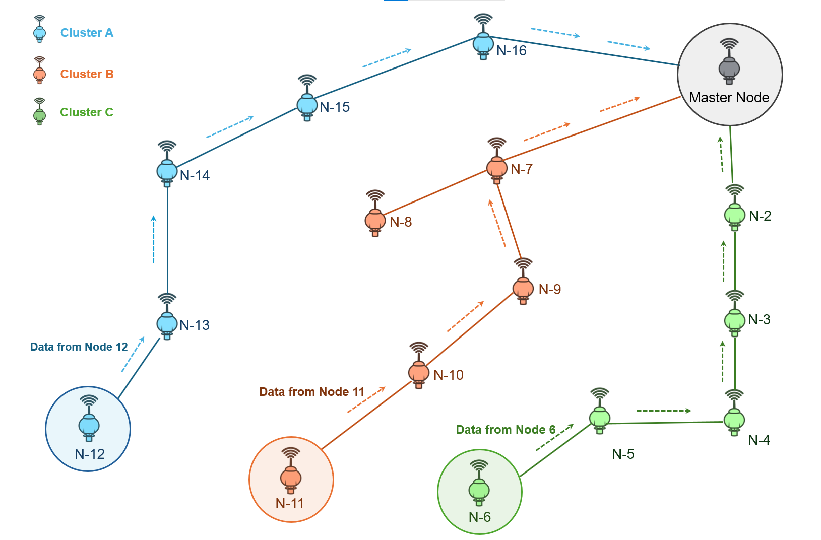
Cluster A: Underwater nodes 12, 13, 14, 15, 16.
Cluster B: Underwater nodes 11, 10, 9, 8, 7.
Cluster C: Underwater nodes 6, 5, 4, 3, 2.
Master Node: Node 1, responsible for collecting data from all the clusters.
The network is configured with static routing to ensure data transfer from sensor nodes to the master node. We assume an ideal channel with no pathloss.
Device Configuration
| Device Properties | |
|---|---|
| Mac Layer | |
| Protocol | Slotted Aloha |
| Slot Length(\(\mu\)s) | 525420 |
| Phy Layer | |
| Source Level (dB//1\(\mu\)Pa) | 190 |
| Modulation | QPSK |
| Data Rate (kbps) | 20 |
| Power | |
| Power source | Battery |
| Initial energy (mAH) | 10416 |
| Transmitting current (mA) | 6250 |
| Idle mode current (mA) | 1.6 |
| Voltage (v) | 48 |
| Receiving current (mA) | 37.5 |
In our project, we use a data rate of 20 Kbps, whereas at the time of publication of reference [9], the modems supported data rates of 10s to 100s of bits per second. Consequently, the network in the current NetSim simulation can support a much higher traffic load. Therefore, while we expect different numerical results when comparing the outcomes, we anticipate observing similar trends to those reported in [9].
Slot Length Calculation
This is a global parameter applicable to all UWAN devices. As a starting step, estimate the transmission time \({T}_{tx}\), which would be
\[\begin{equation} {T}_{tx}\left(\mu s\right)=\frac{\left({L}_{pkt}+OH\right)\times 8}{PHYRate} \end{equation}\]
where \({L}_{pkt}\) is the application layer packet size, \(OH\) is the overheads of all layers which is equal to 28B, and \(PHYRate\) is the data rate set in the PHY layer. Next, the propagation delay, \(\Delta\) is computed as \(\Delta =\frac{d}{{c}_{sound}},\) where \(d\) is the distance between the transmitter and the receiver. Thus, the ideal slot length should be
\[\begin{equation} {L}_{slot}= \frac{\left({L}_{pkt}+OH\right)\times 8}{PHYRate}+\frac{d}{{C}_{sound}} \end{equation}\]
In our scenario \({L}_{pkt}=14B\) and \(PHYRate=20\ Kbps\) which leads to \({T}_{tx}=16{,}800\ \mu s\). Then using \(t=\frac{25}{10}=2.5,\) \(z=50\), and \(S=35\) - where t is one-tenth of the temperature of the water in degrees Celsius, z is the depth in meters and S is the salinity of the water - we get \({c}_{sound}=2799.33\ m/s\).
When the transmitter receiver distance is \(d=1423.79\ m\), the propagation delay,
\[\begin{equation} \Delta =\frac{1423.79}{2799.33}= 508618.13\ \mu s. \end{equation}\]
Substituting all these, we see that the ideal slot length (when \(d=1423.79\)) would be
\[\begin{equation} {L}_{slot}={T}_{tx}+\Delta =16{,}800+508618.13=525420\ \mu s \end{equation}\]
NOTE: The slot length is set based on the largest Tx-Rx distance i.e., from node 2 to Master node 1
Application Configuration
Create a three CBR Application from the source nodes (12, 11, 6) to the Destination (Node 1) with a packet size of 14 bytes each and we will vary the inter arrival according to the load
| Load (Pkt/sec) | Inter Arrival time | Load (Pkt/sec) | Inter Arrival time |
|---|---|---|---|
| 0.001 | 1000000000 | 0.0095 | 105263157 |
| 0.0015 | 666666666 | 0.01 | 100000000 |
| 0.002 | 500000000 | 0.02 | 50000000 |
| 0.0025 | 400000000 | 0.03 | 33333333 |
| 0.003 | 333333333 | 0.04 | 25000000 |
| 0.0035 | 285714285 | 0.05 | 20000000 |
| 0.004 | 250000000 | 0.06 | 16666666 |
| 0.0045 | 222222222 | 0.07 | 14285714 |
| 0.005 | 200000000 | 0.08 | 12500000 |
| 0.0055 | 181818181 | 0.09 | 11111111 |
| 0.006 | 166666666 | 0.1 | 10000000 |
| 0.0065 | 153846153 | 0.2 | 5000000 |
| 0.007 | 142857142 | 0.3 | 3333333 |
| 0.0075 | 133333333 | 0.4 | 2500000 |
| 0.008 | 125000000 | 0.5 | 2000000 |
| 0.0085 | 117647058 | 0.6 | 1666666 |
| 0.009 | 111111111 |

Simulation results
Post simulation, click on the additional metrics in the simulation results window and scroll down for battery model metrics as shown below.

The transmitting energy, receiving energy, idle energy, and total consumed energy for the Master node, Layer1 Node 7, and Layer2 Node 15 are tabulated in individual tables for different loads.
| Load (Pkt/sec) | Transmit Energy (mJ) | Receive Energy (mJ) | Idle Energy (mJ) | Total Consumed Energy (mJ) |
|---|---|---|---|---|
| 0.001 | 0 | 26307 | 691807 | 718113 |
| 0.0015 | 0 | 40796 | 716045 | 756841 |
| 0.002 | 0 | 55483 | 728281 | 783764 |
| 0.0025 | 0 | 68962 | 735374 | 804336 |
| 0.003 | 0 | 85278 | 739642 | 824919 |
| 0.0035 | 0 | 98271 | 742889 | 841159 |
| 0.004 | 0 | 111749 | 744856 | 856605 |
| 0.0045 | 0 | 125491 | 746883 | 872373 |
| 0.005 | 0 | 140663 | 748698 | 889361 |
| 0.0055 | 0 | 153426 | 748517 | 901943 |
| 0.006 | 0 | 169059 | 749059 | 918118 |
| 0.0065 | 0 | 182570 | 749340 | 931910 |
| 0.007 | 0 | 198170 | 750409 | 948580 |
| 0.0075 | 0 | 211879 | 749936 | 961815 |
| 0.008 | 0 | 223927 | 751157 | 975083 |
| 0.0085 | 0 | 235974 | 750280 | 986253 |
| 0.009 | 0 | 249913 | 750492 | 1000405 |
| 0.0095 | 0 | 266096 | 750124 | 1016220 |
| 0.01 | 0 | 281333 | 749353 | 1030686 |
| 0.02 | 0 | 575793 | 740784 | 1316577 |
| 0.03 | 0 | 854663 | 731155 | 1585818 |
| 0.04 | 0 | 1202139 | 715724 | 1917863 |
| 0.05 | 0 | 1619240 | 698524 | 2317764 |
| 0.06 | 0 | 2258239 | 670898 | 2929137 |
| 0.07 | 0 | 3088371 | 636044 | 3724415 |
| 0.08 | 0 | 3558266 | 616165 | 4174430 |
| 0.09 | 0 | 3645710 | 612425 | 4258136 |
| 0.1 | 0 | 3724541 | 608901 | 4333442 |
| 0.2 | 0 | 3488490 | 619132 | 4107622 |
| 0.3 | 0 | 3471500 | 619817 | 4091317 |
| 0.4 | 0 | 3377058 | 622000 | 3999057 |
| 0.5 | 0 | 3479548 | 619362 | 4098910 |
| 0.6 | 0 | 3542675 | 616830 | 4159505 |
| Load (Pkt/sec) | Transmit Energy (mJ) | Receive Energy (mJ) | Idle Energy (mJ) | Total Consumed Energy (mJ) |
|---|---|---|---|---|
| 0.001 | 1312019 | 10995 | 691065 | 2014079 |
| 0.0015 | 1908392 | 15224 | 716275 | 2639890 |
| 0.002 | 2504764 | 20298 | 729141 | 3254203 |
| 0.0025 | 3339685 | 24527 | 735728 | 4099940 |
| 0.003 | 4174607 | 30447 | 740628 | 4945682 |
| 0.0035 | 4770979 | 35522 | 743810 | 5550311 |
| 0.004 | 5605901 | 42288 | 745971 | 6394159 |
| 0.0045 | 6202273 | 46516 | 748664 | 6997454 |
| 0.005 | 7037194 | 50745 | 749118 | 7837057 |
| 0.0055 | 7752841 | 54974 | 750409 | 8558223 |
| 0.006 | 8349214 | 60048 | 751573 | 9160835 |
| 0.0065 | 9064860 | 65969 | 751702 | 9882531 |
| 0.007 | 9780507 | 74426 | 752167 | 10607100 |
| 0.0075 | 10496154 | 78655 | 752933 | 11327742 |
| 0.008 | 11092527 | 89650 | 754046 | 11936222 |
| 0.0085 | 11688899 | 93878 | 753350 | 12536127 |
| 0.009 | 12285271 | 98953 | 753788 | 13138012 |
| 0.0095 | 12881644 | 103182 | 753777 | 13738603 |
| 0.01 | 13478016 | 107410 | 753323 | 14338750 |
| 0.02 | 27790954 | 219049 | 748891 | 28758894 |
| 0.03 | 42700264 | 317612 | 741797 | 43759672 |
| 0.04 | 59517965 | 434000 | 732687 | 60684652 |
| 0.05 | 76335667 | 584479 | 723131 | 77643277 |
| 0.06 | 108062678 | 712383 | 708987 | 109484048 |
| 0.07 | 147542531 | 1025897 | 686074 | 149254502 |
| 0.08 | 170443231 | 1274352 | 669363 | 172386946 |
| 0.09 | 201454596 | 1458335 | 653378 | 203566309 |
| 0.1 | 204078634 | 1622671 | 645366 | 206346672 |
| 0.2 | 236521293 | 2101952 | 617747 | 239240991 |
| 0.3 | 243319938 | 1984392 | 620982 | 245925312 |
| 0.4 | 229841922 | 1961101 | 625426 | 232428449 |
| 0.5 | 211473652 | 1905802 | 631998 | 214011452 |
| 0.6 | 255128111 | 2118476 | 612071 | 257858659 |
| Load (Pkt/sec) | Transmit Energy (mJ) | Receive Energy (mJ) | Idle Energy (mJ) | Total Consumed Energy (mJ) |
|---|---|---|---|---|
| 0.001 | 1360311 | 8456 | 690873 | 2059639 |
| 0.0015 | 1943301 | 14093 | 716389 | 2673783 |
| 0.002 | 2526291 | 17475 | 728847 | 3272613 |
| 0.0025 | 3303611 | 20858 | 736534 | 4061003 |
| 0.003 | 3789436 | 24240 | 741228 | 4554905 |
| 0.0035 | 4469592 | 27059 | 744525 | 5241176 |
| 0.004 | 4955417 | 29877 | 746823 | 5732117 |
| 0.0045 | 5441242 | 34387 | 748685 | 6224314 |
| 0.005 | 6121397 | 37206 | 751498 | 6910101 |
| 0.0055 | 6898718 | 40024 | 751542 | 7690284 |
| 0.006 | 7481708 | 43970 | 751749 | 8277427 |
| 0.0065 | 8161863 | 48480 | 752431 | 8962775 |
| 0.007 | 8647688 | 51862 | 753131 | 9452682 |
| 0.0075 | 9133513 | 55245 | 753387 | 9942145 |
| 0.008 | 9910834 | 58063 | 754561 | 10723458 |
| 0.0085 | 10493824 | 60882 | 754372 | 11309078 |
| 0.009 | 10979649 | 64828 | 754200 | 11798678 |
| 0.0095 | 11562639 | 68210 | 754552 | 12385402 |
| 0.01 | 12048465 | 71593 | 754728 | 12874785 |
| 0.02 | 23513939 | 145440 | 752394 | 24411774 |
| 0.03 | 35076578 | 212523 | 747783 | 36036884 |
| 0.04 | 48874014 | 303846 | 741121 | 49918981 |
| 0.05 | 58292600 | 395733 | 734991 | 59423323 |
| 0.06 | 77508797 | 546810 | 724029 | 78779637 |
| 0.07 | 106500128 | 751442 | 707997 | 107959567 |
| 0.08 | 123932855 | 968475 | 688867 | 125590197 |
| 0.09 | 144988766 | 1032739 | 686546 | 146708050 |
| 0.1 | 158314046 | 1169160 | 676869 | 160160075 |
| 0.2 | 129284179 | 1241880 | 681804 | 131207862 |
| 0.3 | 136798000 | 1231169 | 679611 | 138708780 |
| 0.4 | 140626797 | 1258228 | 678243 | 142563269 |
| 0.5 | 167477286 | 1303889 | 669477 | 169450652 |
| 0.6 | 141795989 | 1167468 | 681776 | 143645234 |
Throughput and Packet collision count
The values for throughput of three applications and packets collided are listed below for different loads:
| Load (Pkt/sec) | Throughput-1 (Mbps) | Throughput-2 (Mbps) | Throughput-3 (Mbps) | Packets Collided |
|---|---|---|---|---|
| 0.001 | 0 | 0 | 0 | 154 |
| 0.0015 | 0 | 0 | 0 | 233 |
| 0.002 | 0 | 0 | 0 | 306 |
| 0.0025 | 0 | 0 | 0 | 374 |
| 0.003 | 0 | 0 | 0 | 439 |
| 0.0035 | 0 | 0 | 0 | 511 |
| 0.004 | 0 | 0 | 0 | 578 |
| 0.0045 | 0.000001 | 0.000001 | 0.000001 | 642 |
| 0.005 | 0.000001 | 0.000001 | 0.000001 | 719 |
| 0.0055 | 0.000001 | 0.000001 | 0.000001 | 782 |
| 0.006 | 0.000001 | 0.000001 | 0.000001 | 843 |
| 0.0065 | 0.000001 | 0.000001 | 0.000001 | 913 |
| 0.007 | 0.000001 | 0.000001 | 0.000001 | 980 |
| 0.0075 | 0.000001 | 0.000001 | 0.000001 | 1052 |
| 0.008 | 0.000001 | 0.000001 | 0.000001 | 1125 |
| 0.0085 | 0.000001 | 0.000001 | 0.000001 | 1194 |
| 0.009 | 0.000001 | 0.000001 | 0.000001 | 1261 |
| 0.0095 | 0.000001 | 0.000001 | 0.000001 | 1331 |
| 0.01 | 0.000001 | 0.000001 | 0.000001 | 1396 |
| 0.02 | 0.000002 | 0.000002 | 0.000002 | 2805 |
| 0.03 | 0.000003 | 0.000003 | 0.000003 | 4167 |
| 0.04 | 0.000004 | 0.000004 | 0.000004 | 5747 |
| 0.05 | 0.000005 | 0.000005 | 0.000005 | 7542 |
| 0.06 | 0.000006 | 0.000006 | 0.000006 | 10088 |
| 0.07 | 0.000006 | 0.000006 | 0.000006 | 14228 |
| 0.08 | 0.000005 | 0.000006 | 0.000006 | 18428 |
| 0.09 | 0.000005 | 0.000006 | 0.000005 | 21346 |
| 0.1 | 0.000004 | 0.000005 | 0.000004 | 24555 |
| 0.2 | 0.000002 | 0.000004 | 0.000003 | 27718 |
| 0.3 | 0.000002 | 0.000004 | 0.000002 | 27771 |
| 0.4 | 0.000002 | 0.000003 | 0.000002 | 28000 |
| 0.5 | 0.000002 | 0.000003 | 0.000002 | 28074 |
| 0.6 | 0.000002 | 0.000004 | 0.000002 | 28143 |
Packets Collision Count

As the load increases, the number of collisions rises sharply until it reaches a plateau. At low loads, the probability of collision is relatively low, and most packets are successfully transmitted. However, as the load increases, the probability of two or more packets being transmitted in the same time slot rises exponentially, leading to a rapid increase in collisions.
NetSim slotted Aloha implementation uses the exponential backoff algorithm when collisions occur. As collisions become frequent at high loads, nodes spend more time in backoff, effectively reducing their transmission attempts and stabilizing the collision rate.
Throughput

The throughput behaviour can be explained by considering both the collision plot and the throughput graphs:
Initial increase: At low loads, throughput increases as more packets are successfully transmitted with relatively few collisions.
Peak throughput: The throughput reaches a maximum at an optimal load point (around 0.05–0.07 packets/sec). This represents the best balance between channel utilization and collision avoidance.
Sharp decline: As load increases beyond the optimal point, we see a sharp rise in collisions (from the collision plot). This leads to a rapid drop in throughput because:
More transmission attempts result in collisions rather than successful transmissions.
Colliding packets waste channel capacity without contributing to throughput.
The exponential backoff algorithm causes nodes to wait longer before retransmitting, reducing overall transmission attempts.
Gradual stabilization: The collision plot shows a plateau at higher loads, but throughput continues to decrease slightly or stabilize at a lower level. This occurs because:
The network is saturated with collisions.
Most transmission attempts fail due to collisions.
The backoff algorithm limits new transmission attempts.
The actual number of successful transmissions becomes a small fraction of the total load.
Differences between applications:
Applications 1 and 3 use routes with 4 hops and show similar throughput patterns. They experience more throughput degradation at high loads as compared to application 2 due to longer paths.
Application 2 uses a route with only 3 hops and sees better throughput, at higher loads. This is because of the shorter path length, which reduces the overall collision probability because each additional hop increases the likelihood of collisions and packet loss.
The throughput differences among applications stem from cross layer interactions of routing path lengths and the slotted Aloha MAC layer’s behaviour under varying loads.
Master Node 1 Energy Consumption
See Figure 6
The transmission energy from the master node will be zero because no transmission is occurring from the master node.
As the load increases, the number of collisions initially rises rapidly but flattens out. Although the number of successfully received packets decreases, the node continues to receive collided packets. In the NetSim energy model, note that energy is expended in receiving these collided packets. However, once received, the node cannot decode the packets that have undergone collisions.
The idle energy remains significant throughout all loads, though it slightly decreases at higher loads. This is because more energy is being consumed in receiving packets, leaving less time for the node to be idle.

The total consumed energy initially increases with network load, primarily due to the rise in receiving energy, and then flattens out.
Layer-1 Device – Node 7, Energy Consumption
See Figure 7
The transmitting energy for Layer 1 Node 7 increases significantly with the network load as it relays packets of Application 2 to the master node.
The receiving energy also increases with load. This reflects its role in receiving packets that it must then forward to the master node.
The idle energy remains relatively stable but shows a slight decrease at higher loads. This is due to the node spending more energy on transmission and reception rather than staying idle, at higher loads.

The total consumed energy increases with the network load, driven by the substantial rise in both transmitting and receiving energies.
These plots reflect Node 7’s active role in relaying traffic from outer layers to the master node.
Layer-2 Device – Node 15 Energy Consumption
See Figure 8
The curves depicted in the four panels in Figure 8 closely resemble those in Figure 7 with the only distinction being slightly lower values. This difference arises because: Node 15 serves as a relay for Application 1, while Node 7 relays for Application 2. Application 1 sees lower throughput compared to Application 2 due to its longer path (4 hops versus 3 hops). Consequently, Node 15 relays fewer packets than Node 7, resulting in reduced transmit and receive energy consumption. This, in turn, leads to lower total energy consumption for Node 15.
