Model Features
Under the Physical Layer, two types of links are modeled in the Satellite communication system.
Abstract Link
Satellite Link
Abstract Link Model
The Abstract Link represents an idealized communication channel model implemented under the Physical Layer. It applies to both the Forward and Return directions. Unlike the Satellite Link, with Abstract Link NetSim does not perform link-budget or radio-frequency calculations.
Configurable Parameters
The Abstract Link behaviour is characterized by a small set of user-specified parameters that determine the resulting throughput, delay, etc.
Link Speed (Mbps)
Defines the constant data rate available on the link and is used to compute the packet transmission time.
Bit Error Rate (BER)
Represents the probability of bit errors occurring during transmission over the communication link.
Propagation Delay (ms)
Represents the signal propagation delay, which can be either:
Auto Computed: Calculated automatically based on device distance and the speed of light.
Fixed: A constant delay value entered by the user.
Satellite Link Model
The Satellite Link implements a detailed physical layer model that captures RF propagation characteristics such as free-space pathloss, antenna gain, EIRP, additional losses, noise figure, interference (CIR), and SNR/SINR-based adaptive and fixed modulation and coding.
With this model NetSim performs link-budget-based calculations to determine received signal strength and signal quality parameters such as SNR, and SINR. In the current implementation, SNR-based link-budget computation is applied only for the service links (User-terminal (UT) \(\leftrightarrow\) Satellite).
UT \(\rightarrow\) Satellite (Uplink)
Satellite \(\rightarrow\) UT (Downlink)
For the feeder links (i.e., Gateway \(\leftrightarrow\) Satellite), SNR calculation is not applied. These links operate using the same link-speed and propagation delay values, computed for the service link.
TDMA Forward Link and MF TDMA Return Link

In NetSim, a Forward link is defined as the direction from Satellite Gateway to Satellite to UT Node / UT Router. A Return link is defined as the direction from the UT Node / UT Router to Satellite to the Satellite Gateway.
The protocol operating in the Forward link is Time Division Multiple Access (TDMA). The protocol operating in the Return link is Multi Frequency Time Division Multiple Access (MF-TDMA).
Both the Forward link and Return link transmissions in NetSim are modeled as Layer-2 transmissions. The framing is as explained in the subsequent paragraph.
Each Super Frame is composed of a number of Frames. This is taken as a user input, given by the attribute Frame count in Superframe available in Satellite \(\rightarrow\) Interface Satellite \(\rightarrow\) Physical Layer properties.
Downlink MAC Scheduling
The satellite MAC implements a beam-based, event-driven TDMA scheduling mechanism with adaptive modulation and coding (AMC).
Scheduling decisions are made dynamically at run time, and transmission timing is driven by frame completion events, not by fixed time boundaries.
Each beam operates as an independent scheduler, allowing parallel transmissions without global synchronization.
Beam Formation
Each UT is associated with a beam; this selection is based on maximum SINR.
Each beam maintains its list of UTs.
Beam-wise Scheduling
Each beam operates as an independent TDMA scheduler.
Frame transmissions occur independently at each beam.
Scheduling decisions within one beam do not affect other beams.
Frame Allocation and Round Robin Scheduling
Each transmitted frame is assigned to exactly one UT.
Frame assignment follows a round-robin (RR) policy within the beam.
The round-robin state is maintained per beam, not globally.
Scheduling Flow (Per Beam)
A frame is scheduled for a UT.
The frame is transmitted.
At frame completion, the next frame for the same beam is immediately scheduled.
The next UT is selected using round-robin rotation.
This creates a continuous transmission chain per beam.
Packet Packing within Frames:
Once a frame is assigned to a UT buffer, packets are packed into the frame.
Packing Rules
Packets are packed sequentially from the buffer head (FIFO).
Packet size is evaluated in bits.
A packet is included only if it fully fits within the remaining frame capacity.
Partial packet transmission is not supported.
Packing stops when:
The next packet exceeds the remaining frame capacity.
The buffer becomes empty.
At the end of packing, the frame contains only the packets that fully fit within its capacity.
Frame Length and Payload Capacity Computation
The total frame size is fixed as per DVB-S2 specifications
\[\mathit{Frame\_Bits} = 64800\]
Symbol rate is the effective bandwidth that we set in the GUI
Based on the selected modulation and coding
Number of Symbols per Frame
\[\mathit{SymbolsPerFrame} = \mathit{Frame\_Bits} / \mathit{Mod\_Bits}\]
Frame Duration
\[\mathit{FrameDuration} = (\mathit{SymbolsPerFrame} / \mathit{SymbolRate})\]
Usable Payload Capacity
\[\mathit{PayloadBits} = \mathit{Frame\_Bits} \times \mathit{CodingRate}\]
Impact of SINR (Adaptive MCS)
Higher SINR results in the selection of higher-order modulation and coding schemes. This leads to:
Shorter frame duration
Higher payload capacity
Lower SINR results in longer frame durations and reduced payload capacity.
Frame duration directly influences superframe timing.
NOTE: Uplink scheduling is not implemented currently.
Modulation and coding (MODCOD) schemes selection
The Modulation and Coding Scheme (MCS) determines the combination of modulation order and coding rate used in the physical layer for both the Forward and Return links.
NetSim supports two MCS configuration modes: Fixed MCS and Adaptive MCS.
Fixed MCS Mode
In Fixed MCS mode, the modulation and coding rate remain constant throughout the simulation.
The user selects the desired modulation type (e.g., QPSK, 8PSK, 16APSK, etc.) and coding rate from the GUI.
The selected MCS values are applied to all devices, irrespective of variations in the channel or SNR conditions.
Modulation and coding schemes supported:
QPSK with coding rates 1/3, 1/2, 1/4, 2/5, 3/5, 2/3, 3/4, 4/5, 5/6, 8/9, 9/10
8PSK with coding rates 3/5, 2/3, 3/4, 5/6, 8/9, 9/10
16APSK with coding rates 2/3, 3/4, 4/5, 5/6, 8/9, 9/10
16QAM with coding rates 3/4, 5/6
32APSK with coding rates 3/4, 4/5, 5/6, 8/9, 9/10
These modulation and coding rates are specified in Table 12 on page 32 of the ETSI EN 302 307 – European Standard.
Adaptive MCS Mode
In Adaptive MCS mode, the physical layer dynamically adjusts the modulation and coding rate based on the Signal-to-Noise Ratio (SNR) calculated from the link-budget model.
MCS Configuration files
NetSim uses external configuration files to define the mapping between SNR and the corresponding Modulation and Coding Scheme (MCS).
Separate CSV files are used for the Forward and Return links:
ForwardLink_Modulation.csv
ReturnLink_Modulation.csv
The format of the CSV files is as shown below:
Index, Modulation, Coding Rate and Spectral Efficiency
| Modulation | CodingRate | SpectralEfficiency |
|---|---|---|
| QPSK | 0.333333 | 0.56 |
| QPSK | 0.5 | 0.87 |
| QPSK | 0.666667 | 1.26 |
| QPSK | 0.75 | 1.42 |
| QPSK | 0.833333 | 1.6 |
| 8PSK | 0.666667 | 1.7 |
| 8PSK | 0.75 | 1.93 |
| 8PSK | 0.833333 | 2.13 |
| 16QAM | 0.75 | 2.59 |
| 16QAM | 0.833333 | 2.87 |
| Return link Spectral efficiency values | ||
| QPSK | 0.25 | 0.490243 |
| QPSK | 0.333333 | 0.656448 |
| QPSK | 0.4 | 0.789412 |
| QPSK | 0.5 | 0.988858 |
| QPSK | 0.6 | 1.188304 |
| QPSK | 0.666667 | 1.322253 |
| QPSK | 0.75 | 1.487473 |
| QPSK | 0.8 | 1.587196 |
| QPSK | 0.833333 | 1.654663 |
| QPSK | 0.888889 | 1.766451 |
| 8PSK | 0.6 | 1.779991 |
| QPSK | 0.9 | 1.788612 |
| 8PSK | 0.666667 | 1.980636 |
| 8PSK | 0.75 | 2.228124 |
| 8PSK | 0.833333 | 2.478562 |
| 16APSK | 0.666667 | 2.637201 |
| 8PSK | 0.888889 | 2.646012 |
| 8PSK | 0.9 | 2.679207 |
| 16APSK | 0.75 | 2.966728 |
| 16APSK | 0.8 | 3.165623 |
| 16APSK | 0.833333 | 3.300184 |
| 16APSK | 0.888889 | 3.523143 |
| 16APSK | 0.9 | 3.567342 |
| 32APSK | 0.75 | 3.703295 |
| 32APSK | 0.8 | 3.951571 |
| 32APSK | 0.833333 | 4.11954 |
| 32APSK | 0.888889 | 4.397854 |
| 32APSK | 0.9 | 4.453027 |
Adaptive MCS Selection Logic
Obtain the Signal-to-Interference-Noise Ratio (SINR).
Convert SNR from dB to Linear Scale.
\[\begin{equation} SINR_{Linear}=10^{\left(\frac{SINR_{dB}}{10}\right)} \end{equation}\]
Compute Spectral Efficiency (SE)
\[\begin{equation} \text{Spectral Efficiency}=\log_{2}(1+SINR_{Linear}) \end{equation}\]
Select the Appropriate MCS files based on the link direction.
The selected CSV file defines how spectral efficiency maps to the corresponding modulation and coding rate.
The entry with the largest spectral-efficiency threshold that is less than or equal to the computed SE is chosen.
This Adaptive MCS mechanism enables dynamic adjustment of modulation and coding according to real-time channel conditions.
As the SNR increases, higher-order modulation and coding rates are selected to enhance spectral efficiency and throughput.
The modulation, coding rate and spectral efficiency values used in NetSim’s Adaptive MCS configuration are derived from the OpenSAND MODCOD database (https://github.com/CNES/opensand/wiki/acm).
Physical layer framing for forward and return links

Default settings in NetSim
Frame Type: Normal (Options are normal or short)
Satellite PHY
Given below is the data rate calculation methodology for both forward and return links. The parameter values used are the default values in NetSim GUI.
\[\begin{equation} \text{Symbol Rate}=\frac{BW}{(1+(\text{Roll off factor}))} \end{equation}\]
\[\begin{equation} \text{Bit Rate}=\text{Symbol rate}\times \text{Modulation order}\times \text{CodeRate} \end{equation}\]
\[\text{Bandwidth }(Hz)=\text{Frame\_Bandwidth }(Hz)=10^{6}\text{ Hz}\]
\[\text{Central Frequency }(Hz)=\text{Base Frequency }(Hz)+\frac{\text{Bandwidth }(Hz)}{2.0}\]
\[\text{Central Frequency }(Hz)=26\times 10^{9}+ \frac{10^{6}}{2}=2.60005\times 10^{10}\text{ Hz}\]
\[\begin{equation} \text{Effective Bandwidth }(Hz)=\frac{ \text{Carrier Bandwidth }(Hz)}{(\text{RollOffFactor}+1.0)\times (\text{SpacingFactor}+1.0)} \end{equation}\]
\[\text{Effective Bandwidth }(Hz)=\frac{10^{6}}{(1.0+1.0)\times (1.0+1.0)}=25\times 10^{4}\text{ Hz}\]
\[\text{Symbol Rate}=\text{Effective Bandwidth }(Hz)=25\times 10^{4}\text{ Hz}\]
\[\text{Modulation Bits}=2\]
The number of Modulation Bits depends on the modulation scheme per the table below:
| Modulation | Modulation bits |
|---|---|
| QPSK | 2 |
| 8PSK | 3 |
| 16APSK/16QAM | 4 |
| 32APSK | 5 |
Satellite PHY: Land Satellite Channel Model
Propagation
The distance between the ground nodes and the satellite determines the propagation delay and path loss of the radio signal. The distance is computed based on the cartesian distance between the ground nodes and the satellite. NetSim computes the propagation delay of the radio signal traveling from the source node to the destination node at the speed of light. The propagation model calculates the weakening of the radio signal as it propagates from the source node per the pathloss and fading model.
Earth fixed spot beams and cells
NetSim provides three methods for configuring satellite beams:
Standard setup:
The Standard Setup option allows users to quickly configure satellite beams using predefined parameters without manually entering beam coordinates or importing external files. NetSim automatically calculates the beam geometry, radius, and coverage area based on the selected inputs.
Number of spot beams.
NetSim can presently support configurations of 1, 7, or 19 spot beams.
The 7-cell setup consists of a central hexagonal cell surrounded by 6 adjacent cells.
The 19-cell configuration has two layers of surrounding cells around a central hexagonal cell.
NetSim will automatically compute the tessellated beams (cells) based on number of spot beams.
User-defined beam configuration:
This option allows users to upload an Excel/CSV file containing beam parameters such as beam count, Frequency reuse, Satellite altitude (km), HPBW (theta), Aperture radius (m), Band, Beam centers, Antenna model and Beam radius (km) details instead of relying on automatic or standard setup.

Manual Placement:
The Manual Placement option allows complete user control over beam locations, coverage regions, and satellite altitude. Unlike the Standard Setup or CSV Upload options, no beam parameters are auto-generated. This mode is intended for advanced users who want full flexibility in defining exact beam geometry.
Link budget calculations
UT is sending to Satellite:
The carrier-to-noise ratio, CNR in dB, is calculated per the equation described in TR 38.821 Section 6.1.3.1, given by
\[\begin{equation} CNR=EIRP - \text{MaxAntennaGain} + \text{AngularGain} + Rx\frac{G}{T} - k - PL_{FS} - PL_{AD} - B \label{eq:cnr} \end{equation}\]
where:
\(CNR\) is the carrier to noise ratio (also sometimes termed as SNR or signal to noise ratio) in dB
\(EIRP\) is the effective isotropic radiated power in dBW
\(Rx\frac{G}{T}\) is the antenna-gain-to-noise temperature in dB/K of the receiver
\(k\) is the Boltzmann constant with the value of \(-228.6\) dBW/K/Hz
\(PL_{FS}\) is the free space path loss (FSPL) in dB
\(PL_{AD}\) is the additional loss in dB
\(B\) is the channel bandwidth in dBHz (i.e., \(10\log_{10}(BW),\) where \(BW\) is bandwidth in Hz)
\(Rx\frac{G}{T}\) is obtained using the expression
\[\begin{equation} Rx\frac{G}{T}=G_{rx}-N_{f}-10\log_{10}\left(T_{0}+\left(T_{a}-T_{0}\right)\times 10^{-0.1\times N_{f}}\right) \label{eq:rgt} \end{equation}\]
where:
\(G_{rx}\) is the receive antenna gain in dBi.
\(N_{f}\) is the noise figure in dB
\(T_{0}\) is the ambient temperature in degrees Kelvin, set to \(290\) by default
\(T_{a}\) is the antenna temperature in degrees Kelvin. \(T_{a}=150\)
The \(CNR\) expression is used in both directions i.e., terrestrial to satellite and satellite to terrestrial.
Satellite is sending to the UT:
\[\begin{equation} CNR=EIRP - \text{MaxAntennaGain} + \text{AngularGain} + \text{UTRx\_Gain} - k - PL_{FS} - PL_{AD} - B \end{equation}\]
Elevation angle:
\[\begin{equation} \alpha = \sin^{-1}\left(\frac{D}{R_u \cdot L}\right) \end{equation}\]
Where, \[\begin{equation} R_u = \sqrt{x_{ue}^{2} + y_{ue}^{2} + z_{ue}^{2}} \end{equation}\]
\[\begin{equation} L = \sqrt{(x_{sat} - x_{ue})^{2} + (y_{sat} - y_{ue})^{2} + (z_{sat} - z_{ue})^{2}} \end{equation}\]
\[\begin{equation} D = \sqrt{(x_{sat} - x_{ue})\cdot x_{ue} + (y_{sat} - y_{ue})\cdot y_{ue} + (z_{sat} - z_{ue})\cdot z_{ue}} \end{equation}\]
EIRP calculations:
In NetSim’s satellite model, the method of computing EIRP depends on the link direction:
Forward Link
In the Forward Link, the satellite transmits toward the user terminal (UT).
The EIRP is defined based on the EIRP Density and the allocated bandwidth of the carrier
\[\begin{equation} EIRP\;[\text{dBW}]= \text{EIRPDensity}\;[\text{dBW/MHz}]+10\log_{10}(BW\;[\text{MHz}]) \end{equation}\]
Return link
In the Return Link, the user terminal (UT) transmits toward the satellite.
The EIRP is computed from the transmit power and the Receive antenna gain of the UT.
\[\begin{equation} EIRP\;[\text{dBW}]= P_{tx}\;[\text{dBm}]-30+G_{Rx}\;[\text{dBi}] \end{equation}\]
SNR - BER Calculation
The Signal-to-Noise Ratio (SNR) is calculated separately for each hop of every link.
SNR-based Bit Error Rate (BER) computation is applied only for the UT–Satellite and Satellite–UT links.
NetSim provides three options for BER.
Model Based: The BER is then calculated for each link based on the SNR. Please see Propagation-Models.pdf document for detailed information on BER calculation.
Fixed: the BER value can be input in the GUI. If this option is chosen, the SNR (derived from propagation model) is not used.
File Based: SNR – BER table should be provided in a file per the format given below. This table should be in increasing order of SNR. The SNR is calculated by NetSim from the RF propagation model. For this SNR, the appropriate BER is selected from this table. BER is 1.0 for any SNR value below SNR1, and BER is 0.0 for any SNR greater than SNRn.
SNR1, BER1
SNR2, BER2
...
SNRn, BERn
NOTE: Users can enable the Satellite Propagation Log to see the SNR calculated from RF propagation model and then choose appropriate entries of SNR, BER values into the BER-File to see the impact on throughput.
Pathloss Model – Friis Free Space Propagation
The free space propagation model is used to predict received signal strength when the transmitter and receiver have a clear, unobstructed line-of-sight path between them. Satellite communication systems and microwave line-of-sight radio links typically undergo free space propagation. The mathematical expression for free-space path loss is given by the Friis Free-Space Equation:
\[\begin{equation} PL_{FS}= 20\log_{10}\left(\frac{4\pi d}{\lambda }\right) \label{eq:fspl} \end{equation}\]
Where \(\lambda =\frac{c}{f},\)
\(d\) is the slant height in meters,
\(\lambda\) is the wavelength in meters.
Fading model
NetSim uses a 3-state (state 1, state 2 and state 3) Markov model to simulate fading.
The conditional probabilities of state \(s_{n+1}\) given the state \(s_{n}\) are described by state transition probabilities \(p_{ij}\)
Where \(S_{1}\), \(S_{2}\), \(S_{3}\) denote respective channel states, \(P_{ij}\) is the probability the Markov process goes from state \(i\) to state \(j\).

The switching among each state is described by a transition matrix P, which is
\[\begin{equation} P= \begin{pmatrix} p_{11} & p_{12} & p_{13} \\ p_{21} & p_{22} & p_{23} \\ p_{31} & p_{32} & p_{33} \end{pmatrix} \end{equation}\]
Each state of the three states of the Markov model obeys the Loo distribution with different parameters, while the state transition is modeled as a first-order Markov random process.
The Loo distribution considers the received signal as a sum of two signal components. A log-normally distributed direct signal expresses the slow fading component corresponding to varying shadowing conditions of the direct signal. A Rice distribution characterizes the fast-fading component due to multipath effects.
The Loo parameter triplet consists of the mean, the standard deviation for the log-normally distributed direct signal, and the average multipath power.
\[\begin{equation} N(\mu , \sigma^{2})+R \end{equation}\]
Depending on the current state interval and on the environment of the terminal, a new random Loo parameter triplet is generated. The output of the channel model is a time-series of the received signal in the form of a complex envelope.
And finally, the model computes the Loo distributed time-series including Doppler shaping for every new state interval, which is the output of the proposed LMS channel model.

Antenna Models
TR 38.811 Antenna model
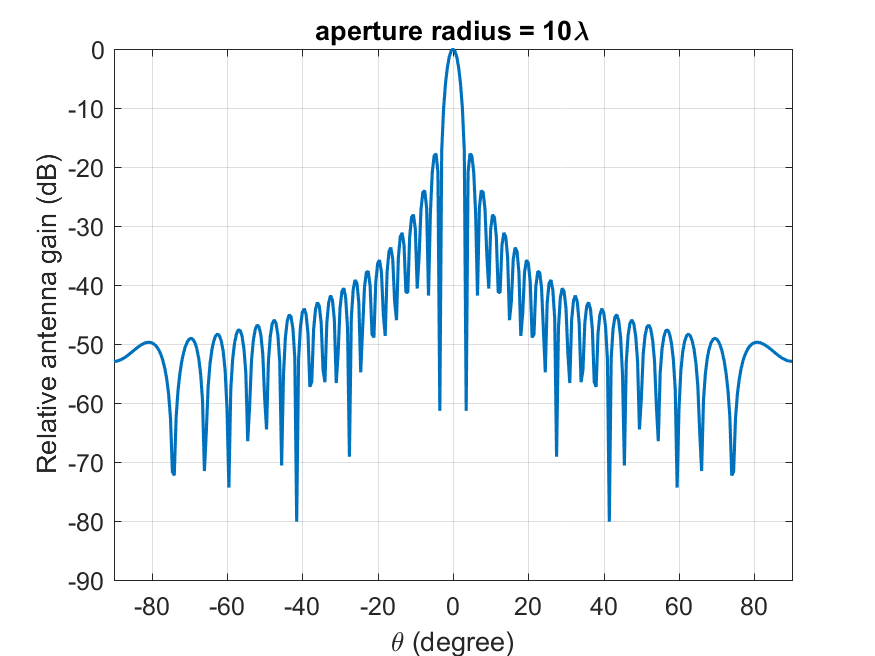
The normalized antenna gain pattern, corresponding to a typical reflector antenna with a circular aperture, is considered
\[\begin{equation} G(\theta) = \begin{cases} 1 & \text{for } \theta = 0 \\[6pt] 4\left|\dfrac{J_{1}(ka\sin\theta)}{ka\sin\theta}\right|^{2} & \text{for } 0 < |\theta| \leq 90^{\circ} \end{cases} \label{eq:tr38811} \end{equation}\]
where \(J_1(x)\) is the Bessel function of the first kind and first order with argument \(x\), \(a\) is the radius of the antenna’s circular aperture, \(k =\frac{2\pi f}{c}\) is the wave number, \(f\) is the frequency of operation, \(c\) is the speed of light in a vacuum and \(\theta\) is the angle measured from the boresight of the antenna’s main beam. Note that \(ka\) equals the number of wavelengths on the circumference of the aperture and is independent of the operating frequency. The above expression provides the gain in linear scale and it needs to be converted to dB scale. The normalized gain pattern for \(a = 10\frac{c}{f}\) (aperture radius of 10 wavelengths) is shown below
ITU-R S.672 Antenna model
To model the off-axis behavior of satellite antennas, the ITU-R S.672 recommendation specifies that, for single-feed circular or elliptical beam spacecraft antennas operating in the fixed-satellite service (FSS), the following radiation pattern should be used as the design objective outside the coverage area.
\[\begin{align} G(\psi) &= G_m - 3 \left(\frac{\psi}{\psi_b}\right)^{\alpha} \;\text{[dBi]} &\text{for } \psi_{b} \leq \psi \leq a\psi_b \label{eq:itu1}\\ G(\psi) &= G_m + LN + 20\log(z) \;\text{[dBi]} &\text{for } a\psi_b < \psi \leq 0.5b\psi_{b} \label{eq:itu2a}\\ G(\psi) &= G_m + LN \;\text{[dBi]} &\text{for } 0.5b\psi_{b} < \psi \leq b\psi_{b} \label{eq:itu2b}\\ G(\psi) &= X - 25 \log \psi \;\text{[dBi]} &\text{for } b\psi_{b} < \psi \leq Y \label{eq:itu3}\\ G(\psi) &= LF \;\text{[dBi]} &\text{for } Y < \psi \leq 90^{\circ} \label{eq:itu4a}\\ G(\psi) &= LB \;\text{[dBi]} &\text{for } 90^{\circ} < \psi \leq 180^{\circ} \label{eq:itu4b} \end{align}\]
Where: \[\begin{equation} X = G_m + LN + 25 \log(b\psi_{b}) \quad\text{and}\quad Y = b\psi_{b} \cdot 10^{0.04(G_m + LN - LF)} \end{equation}\]
\(G(\psi):\) gain at the angle \(\psi\) from the main beam direction (dBi)
\(G_m:\) maximum gain in the main lobe (dBi)
\(\psi_{b}\): one-half the 3 dB beamwidth in the plane of interest (3 dB below \(G_m\)) (degrees)
\(LN\): near-in-side-lobe level in dB relative to the peak gain required by the system design
\(LF = 0\) dBi: far side-lobe level (dBi)
\(z\): (major axis/minor axis) for the radiated beam
\(LB\): \(15 + LN + 0.25 G_m + 5 \log z\) dBi or \(0\) dBi whichever is higher
| \(LN\,(dB)\) | \(a\) | \(b\) | \(\alpha\) |
|---|---|---|---|
| \(-20\) | \(2.58 \cdot \sqrt{(1 - \log(z))}\) | 6.32 | 2 |
| \(-25\) | \(2.58 \cdot \sqrt{(1 - 0.8 \cdot \log(z))}\) | 6.32 | 2 |
The numeric values of \(a\), \(b\), and \(\alpha\) for \(LN = -20\) dB and \(-25\) dB side-lobe levels are given in the above table.
Off Boresight Angle Calculation
Conceptually, the off-boresight angle, \(\theta\), in the antenna gain formula is defined as the angle between two vectors: one along the boresight of the beam (i.e., from the satellite to the beam centre, which corresponds to the sub-satellite nadir point), and the other from the satellite to the UE. In NetSim, \(\theta\) is computed as the arccosine of the normalized dot product of these two vectors.
Standard ENU-Based Look Angle Computation (Satellite to Earth)
This section describes the standard ENU (East–North–Up) method for computing satellite look angles (azimuth and elevation) as seen from an earth station (user terminal).
Notation
\(\varphi_{t}\) : Latitude of earth station (degrees)
\(\lambda_{t}\) : Longitude of earth station (degrees)
\(H_{t}\) : Altitude of earth station above sea level (km)
\(\varphi_{s}\) : Latitude of satellite (degrees)
\(\lambda_{s}\) : Longitude of satellite (degrees)
\(H_{s}\) : Altitude of satellite above sea level (km)
Step 1: Convert Geodetic Coordinates to ECEF
Convert both earth station and satellite geodetic coordinates to Earth-Centered Earth-Fixed (ECEF) Cartesian coordinates.
WGS-84 ellipsoid constants
WGS-84 defines the Earth as an oblate ellipsoid with:
Semi-major axis (equatorial radius):
\[a = 6378137.0 \text{ m}\]
Flattening:
\[f = \frac{1}{298.257223563}\]
First eccentricity squared:
\[e^{2}=2f-f^{2}\]
Numerically:
\[e^{2} \approx 0.00669437999014\]
Prime vertical radius of curvature
\[N(\phi) = \frac{a}{\sqrt{1 - e^{2}\sin^{2}(\phi)}}\]
This is to compensate for Earth’s flattening.
ECEF Conversion formulas (WGS-84)
\[X = (N + h)\cos(\phi)\cos(\lambda)\]
\[Y = (N + h)\cos(\phi)\sin(\lambda)\]
\[Z = \left(N(1 - e^{2}) + h\right)\sin(\phi)\]
This gives Earth-Centered Earth-Fixed (ECEF) coordinates:
\(X\) axis: intersection of equator and Greenwich meridian
\(Y\) axis: \(90^{\circ}\) east on equator
\(Z\) axis: North pole
Step 2: Line-of-Sight Vector in ECEF
Compute the line-of-sight (LOS) vector from the earth station to the satellite:
\[\Delta r = r_{s} - r_{t} = (\Delta X, \Delta Y, \Delta Z)\]
Step 3: Rotate LOS Vector into Local ENU Frame
Define the standard ECEF-to-ENU rotation matrix at the earth station latitude \(\varphi_{t}\) and longitude \(\lambda_{t}\):
\[\begin{equation} \begin{bmatrix} E \\ N \\ U \end{bmatrix} = \begin{bmatrix} -\sin(\lambda_{t}) & \cos(\lambda_{t}) & 0 \\ -\sin(\phi_{t}) \cos(\lambda_{t}) & -\sin(\phi_{t}) \sin(\lambda_{t}) & \cos(\phi_{t}) \\ \cos(\phi_{t}) \cos(\lambda_{t}) & \cos(\phi_{t}) \sin(\lambda_{t}) & \sin(\phi_{t}) \end{bmatrix}\begin{bmatrix} \Delta X \\ \Delta Y \\ \Delta Z \end{bmatrix} \end{equation}\]
This yields the local ENU components (\(E\), \(N\), \(U\)) of the satellite relative to the earth station.
Step 4: Slant Range
The straight-line distance between the earth station and the satellite is:
\[\begin{equation} D_{ts}= \sqrt{E^{2}+ N^{2}+ U^{2}} \end{equation}\]
Step 5: Elevation Angle
The elevation angle (above the local horizontal plane) is computed as:
\[\begin{equation} el = \text{atan2}\left(U, \sqrt{E^{2}+ N^{2}}\right) \end{equation}\]
Elevation is in the range \(-90^{\circ}\) to \(+90^{\circ}\).
Step 6: Azimuth Angle
The azimuth angle, measured clockwise from true North, is:
\[\begin{equation} az = \text{atan2}(E, N) \end{equation}\]
The result should be wrapped to the range \(0^{\circ}\)–\(360^{\circ}\).
Step 7: Visibility Check
Given a minimum elevation mask angle (maskAngle):
\[\text{visible} = 1 \quad\text{if } el \geq \text{maskAngle}\]
\[\text{visible} = 0 \quad\text{otherwise}\]
If \(\sqrt{E^{2}+ N^{2}} \approx 0\) (satellite directly overhead), the azimuth is indeterminate.
Frequency Reuse
NetSim supports FR1 (\(N_{reuse}=1\)), FR2 (\(N_{reuse}=2\)), FR3 (\(N_{reuse}=3\)) and FR4 (\(N_{reuse}=4\)) configurations.
With NetSim GUI, users can configure the number of beams (1, 7, and 19) and select the frequency reuse factor (FRF) accordingly. When \(N_{reuse}>1\), NetSim assigns virtual “channel IDs” to the beams. The available resources and bandwidth are then equally divided among the channels. The bandwidth per channel is calculated per the following expression
\[\begin{equation} BW_{channel}= \frac{BW_{Total}}{N_{channels}} \end{equation}\]
Interference models
Exact Geometric Interference
Geometric interference arises when multiple beams sharing the same channel ID overlap, leading to co-channel interference at user terminals. The level of interference is influenced by the number of beams and the configured frequency reuse factor. In FR1, interference occurs from all available beams, whereas in FR2, FR3 and FR4 it is limited to beams using the same channel ID.
CIR-based Interference
Per TR 38.821 section 6.1.3.1 the Carrier-to-noise-and-interference ratio (CNIR) of the transmission link between satellite and UE can be derived by carrier-to-noise ratio (CNR) and carrier-to-interference ratio (CIR) as follows
\[\begin{equation} CNIR\;[\text{dB}]=-10\log_{10}\left(10^{-0.1\cdot CNR\;[\text{dB}]}+10^{-0.1\cdot CIR\;[\text{dB}]}\right) \label{eq:cnir} \end{equation}\]
Carrier-to-Interference Ratio (CIR) is the user input and
CNR (dB) is computed from the link budget, based on EIRP, G/T, path loss and the antenna gain.
Interference power calculations for CIR based Interference
\[\begin{equation} \text{Interference}\;[\text{mW}]=\text{Noise}\;[\text{mW}] \times \left(\frac{CNR\;[\text{mW}]}{CNIR\;[\text{mW}]}-1\right) \end{equation}\]
\[\begin{equation} \text{Interference}\;[\text{dB}]=10\times \log_{10}(\text{Interference}\;[\text{mW}]) \end{equation}\]
Results
Please refer to the NetSim User Manual, section 8, for Results and Analysis.
Satellite Log
NetSim Satellite Log file records UT Satellite association, calculated superframe, frame, slot, bandwidth, etc. This log can be enabled/disabled by going to Plots option and checking/unchecking the Satellite Log option under the Network Logs section as shown below:

A log file specific to satellite communication, is generated post-simulation as shown in the screenshot below.

On opening, the satellite log file would look like the image below.

This file logs details such as
UT – Satellite Gateway association
Calculated Super frame, frame, slot, bandwidth, carrier count etc. for each satellite.
Frame by frame transmissions with time stamps
Satellite Radio Measurements Log
NetSim Satellite Radio Measurements Log file records Time (ms), Transmitter name, Receiver name, Slant height (km), EIRP (dBW), Elevation Angle (\(^{\circ}\)), RXG_T, Pathloss (dB), Fading loss (dB), Additional loss (dB), Total loss (dB), Angular gain (dB), Rx power (dBm), SNR (dB), Thermal noise (dBm), Channel Id, Beam Id, MCS Index and Coding rate. This log can be enabled/disabled by going to Logs option and checking/unchecking the Satellite Radio Measurements Log option under the Network Logs section as shown below:

The Satellite Radio Measurements.csv file will contain the following information:
Time in Milliseconds
Transmitter Name
Receiver Name
Slant height (km)
EIRP (dBW)
Elevation Angle (\(^{\circ}\))
RXG_T
Pathloss (dB)
Fading loss (dB)
Additional loss (dB)
Total loss (dB)
Angular gain (dB)
Rx power (dBm)
SNR (dB)
Interference (dBm)
Thermal noise (dBm)
Channel Id
Beam Id
MCS Index and
Coding rate
Satellite Radio Measurements log files will be available under the Logs in the results window as shown below:

Users can see Tx Power, Rx power, pathloss, fading-loss, Total loss, Thermal noise, and SNR values in the Log files for each forward and return link.

Satellite Beam Association Log
The NetSim Satellite Beam Association Log file is useful for observing the values recorded for each beam, including Time (ms), TX Name, RX Name, EIRP (dBW), Beam Id, Channel Id, Theta (\(^{\circ}\)), Angular Gain, RXG_T (dB), FSPL (dB), Total loss (dB), SNR (dB), Interference (dBm), Interfering Beam Count, MCS Index, and Coding rate. This log can be enabled/disabled by going to Logs option and checking/unchecking the Satellite Beam Association Log option under the Network Logs section as shown below:

Users can see Angular Gain, Interference and SNR values in the Log files for each forward and return link. These parameters are logged separately for each beam.

Omitted Features
Regenerative transponder where the signal is demodulated, decoded, re-encoded and modulated aboard the satellite.
Impact of Rain/Weather on signal propagation
Forward Error Coding in Layer 2
IPv6 Addressing
No support for LEO, MEO