Featured Examples
India region coverage with 16-Beam GEO Satellite with frequency reuse
Open NetSim, Select Examples \(\rightarrow\) Satellite Communication \(\rightarrow\) India region coverage with 16-Beam GEO Satellite with frequency reuse then click on the tile in the middle panel to load the example as shown below.

This example models a GEO satellite at 35,768 km altitude providing coverage over the mainland Indian region (North-East, Andaman & Nicobar & Lakshadweep will be covered in our next iteration) using 16 spot beams. Each beam spans a \(1^{\circ}\) beamwidth (\(\approx\)312 km radius) and serves 100 randomly placed user terminals, for a total of 1600 UTs across the coverage area. The scenario uses the DVB-S2 protocol with ITU-R S.672-4 antenna patterns. Two frequency reuse configurations are compared: FR2 (250 MHz per beam) and FR4 (125 MHz per beam). FR2 offers higher per-beam bandwidth but increased inter-beam interference; FR4 reduces interference at the cost of bandwidth per beam.

The objective is to evaluate the trade-off between these configurations by measuring SINR and throughput distributions, satellite capacity, and spectral efficiency.
Network Scenario
The following network diagram illustrates what the NetSim UI displays when you open the example configuration file. When the example configuration file is opened, NetSim would take some time to load this large scenario. During this time, the UI displays progress information such as the number of devices and applications being loaded.

Orbit
GEO satellite at 35768 km altitude.
Protocol and Beams
DVB-S2
16 spot beams covering the Indian region.
Randomly placed 100 UTs in each beam (total of 1600UTs).
Frequency reuse options: 2 and 4
Antenna
Pattern: ITU S.672-4
EIRP: 54 dBW
Traffic
Unicast downlink traffic to each UT
Objective
Measure the distributions and percentiles of SINR and throughput
Obtain satellite capacity and spectral efficiency
Simulation Setup in NetSim
The satellite is positioned at 82\(^{\circ}\)E, 0\(^{\circ}\) latitude in GEO orbit.
Remote Server, Router, and Gateway are logical constructs for enabling traffic flow; their positions are not physical.
| System Model | |
|---|---|
| Satellite orbit | GEO 35678 km |
| EIRP (dBW) | 54 |
| Frequency Reuse | FR2, FR4 |
| Frequency Band | 11 GHz |
| Bandwidth (MHz) | 250 MHz for each FR2 beam / 125 MHz for each FR4 beam |
| Traffic | Unicast traffic to each UT |
| Antenna pattern | ITU-R S.672-4 |
| Protocol | DVB-S2 |
| UT Height (m) | 1.2 |
| UT RX Antenna Gain (dB) | 40 |
| Number of beams | 16 |
| Beam width | \(1^{\circ}\) |
| MCS selection | Adaptive MCS |
| UT Density | 100 UTs per beam |
| Frame size (bits) | 64,800 |
Simulation time is set to 10 seconds.
Application is configured from the Wired node to each UT with the generation rate set to 5 Mbps per application.
Beam Positions and Frequency Coloring
| Beam ID | Longitude | Latitude |
|---|---|---|
| 1 | 82.50 | 22.50 |
| 2 | 79.94 | 18.27 |
| 3 | 85.06 | 18.27 |
| 4 | 77.24 | 22.41 |
| 5 | 87.76 | 22.41 |
| 6 | 79.78 | 26.68 |
| 7 | 85.22 | 26.68 |
| 8 | 82.50 | 14.08 |
| 9 | 74.82 | 18.14 |
| 10 | 80.04 | 9.84 |
| 11 | 82.50 | 30.92 |
| 12 | 74.35 | 26.48 |
| 13 | 90.65 | 26.48 |
| 14 | 77.49 | 14.03 |
| 15 | 95.53 | 22.41 |
| 16 | 76.84 | 30.80 |


\[\begin{equation} R_{beam}=h\times \tan\left(\frac{\theta}{2}\right), \quad h=35{,}768\text{ km}, \quad \theta =1^{\circ} \end{equation}\]
\[\begin{equation} R_{beam}=312\text{ km}, \quad \text{InterBeamDist}=\sqrt{3}\cdot R_{beam}=540.57\text{ km} \end{equation}\]
Results Summary
Results: FR2
 |
 |
 |
|
| 5% | 50% | 95% | |
|---|---|---|---|
| SINR (dB) | \(-0.55\) | 4.91 | 8.85 |
| UE Thput. (Mbps) | 1.49 | 3.22 | 4.87 |
| Beam Thput. (Mbps) | 223.74 | 317.61 | 480.91 |
Capacity and Efficiency Metrics (FR2):
Satellite capacity = 5199.75 Mbps
Area Traffic capacity:
Number of beams \(= 16\)
Beam radius, \(R\) \(= 312.3\) km
Area per beam (A) \(=\) \(\frac{3\sqrt{3}}{2} R^{2}=253424.62\text{ km}^{2}\)
Total coverage area = \(253424.62\text{ km}^{2}\times 16=4054793.9\) km\(^{2}\)
Area Traffic Capacity \(=1.28\text{ kbps/km}^{2}\)
Average Spectral efficiency (FR2)
System Bandwidth = 500 MHz
Spectral Efficiency
\[\begin{equation} \eta_{system}= \frac{\text{Aggregate Throughput (bps)}}{\text{System Bandwidth }(Hz)}=\frac{5199.75\times 10^{6}}{500\times 10^{6}}=10.39\text{ bits/s/Hz} \end{equation}\]
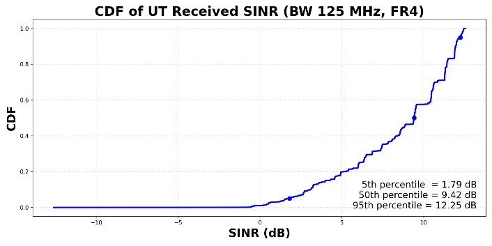
Results: FR4
 |
 |
 |
|
| 5% | 50% | 95% | |
|---|---|---|---|
| SINR (dB) | 1.79 | 9.42 | 12.25 |
| UE Thput. (Mbps) | 0.80 | 2.42 | 4.86 |
| Beam Thput. (Mbps) | 144.37 | 236.04 | 388.62 |
Capacity and Efficiency Metrics (FR4):
Satellite capacity = 4230.56 Mbps
Area Traffic capacity:
Number of beams \(= 16\)
Beam radius, \(R\) \(= 312.3\) km
Area per beam (A) \(=\) \(\frac{3\sqrt{3}}{2} R^{2}=253424.62\text{ km}^{2}\)
Total coverage area = \(253424.62\text{ km}^{2}\times 16=4054793.92\) km\(^{2}\)
Area Traffic Capacity \(=1.04\text{ kbps/km}^{2}\)
Average Spectral efficiency (FR4)
System Bandwidth = 500 MHz
\[\begin{equation} \eta_{system}=\frac{\text{Aggregate Throughput (bps)}}{\text{System Bandwidth }(Hz)}=\frac{4230.56 \times 10^{6}}{500\times 10^{6}}=8.46\text{ bits/s/Hz} \end{equation}\]
5th, 50th, 95th percentile UTs
| (FR 2 case) | 5th percentile | 50th percentile | 95th percentile |
|---|---|---|---|
| Received Signal (dBm) | \(-80.84\) | \(-80.80\) | \(-80.26\) |
| CNR (dB) or C/N | 9.15 | 9.19 | 9.72 |
| Interference Power (dBm) | \(-80.78\) | \(-87.74\) | \(-96.51\) |
| CIR (dB) or C/I | \(-0.07\) | 6.95 | 16.25 |
| CINR (dB) or C/(N+I) | \(-0.55\) | 4.91 | 8.85 |
| Throughput (Mbps) | 1.49 | 3.22 | 4.87 |
The 5% UT is located at the beam edge and subject to interference from other beams.
The 95% UT is near the beam center with very low interference from other beams.
To plot the CDF of SINR per UT and per beam, we considered the metrics.xml file and the Radio Measurements log file.
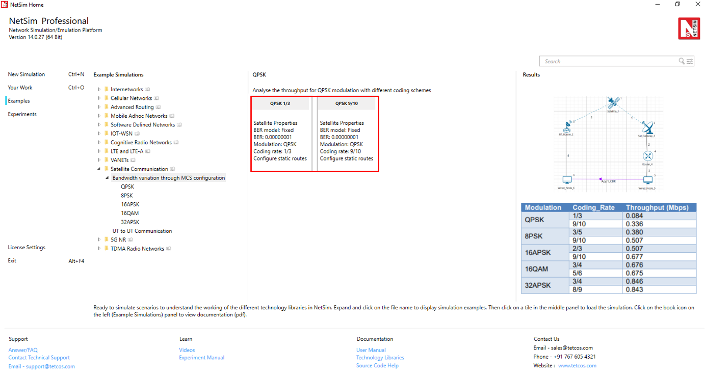
Bandwidth variation through MCS configuration
Open NetSim, Select Examples \(\rightarrow\) Satellite Communication \(\rightarrow\) Bandwidth variation through MCS configuration then click on the tile in the middle panel to load the example as shown below.
The following network diagram illustrates what the NetSim UI displays when you open the example configuration file.

Settings done in example config file:
Set the following property as shown in the table below. To configure it, click on the satellite device, expand the property panel on the right side, and change the property as below.
| Satellite Properties \(\rightarrow\) Interface (Satellite) \(\rightarrow\) Physical Layer \(\rightarrow\) Forward | |
|---|---|
| BER Model | Fixed |
| BER | 0.00000001 |
Click on UT Router and set the following property as shown in below given table.
| UT Router Properties \(\rightarrow\) Interface (Satellite) \(\rightarrow\) Datalink Layer | |
|---|---|
| Gateway | Sat Gateway 2 |
NOTE: For manually configured scenario, the user needs to mention the gateway name for UT nodes under datalink layer.
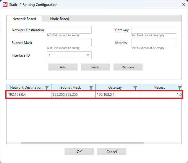
Go to Router 4 properties \(\rightarrow\) Network Layer \(\rightarrow\) Enable – Static IP Route \(\rightarrow\) Click on Static Route IP via GUI.
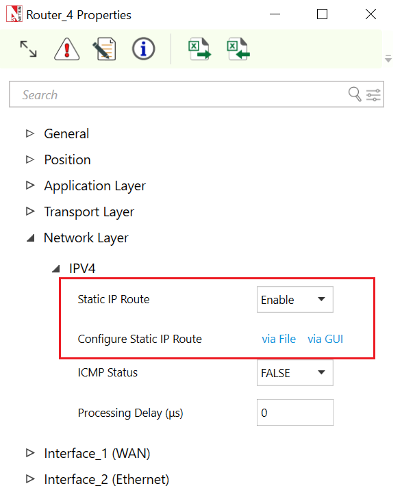
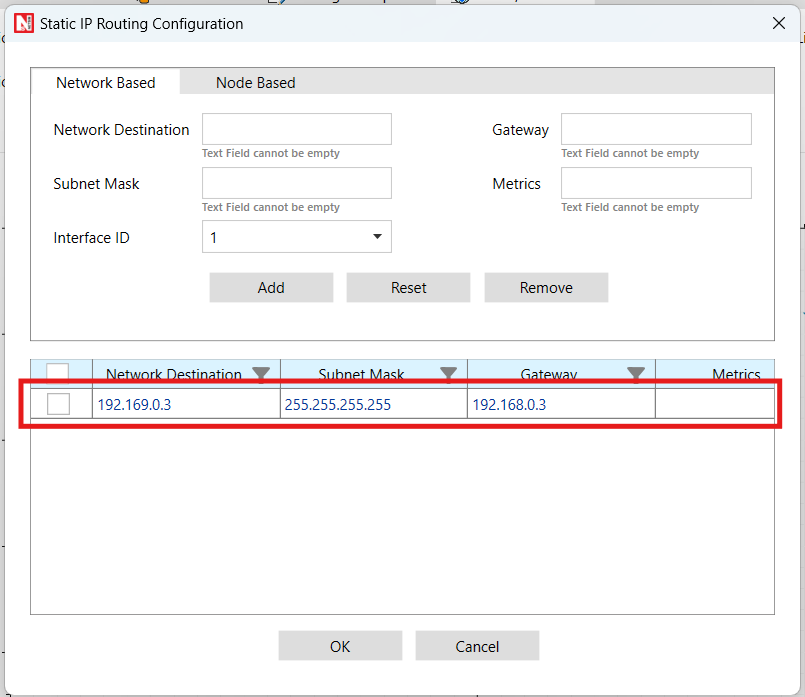
Set the properties in Static Route IP window as per the screenshot below and click on Add. Click on OK.

Go to Sat Gateway 2 properties \(\rightarrow\) Network Layer \(\rightarrow\) Enable – Static IP Route \(\rightarrow\) Configure Static Route IP via GUI. Set the properties in Static Route IP window as per the screenshot below and click on Add. Click on OK.
Go to UT Router 3 properties \(\rightarrow\) Network Layer \(\rightarrow\) Enable – Static IP Route \(\rightarrow\) Configure Static Route IP via GUI. Set the properties in Static Route IP window as per the screenshot below and click on Add. Click on OK.

Create a CBR application from set traffic tab in ribbon on the top between source id 5 to destination id 6 with packet size as 1460 Bytes and Inter Arrival time as 467 \(\mu\)s (Generation Rate = 25 Mbps). Transport Protocol is set to UDP.
Change the Satellite Properties \(\rightarrow\) Interface (Satellite) \(\rightarrow\) Physical Layer \(\rightarrow\) Forward \(\rightarrow\) Modulation and respective coding rates as shown in below Table but the return link uses fixed Modulation \(\rightarrow\) 32APSK and Coding Rate \(\rightarrow\) 3/4.
Run simulation for 10 seconds and observe the result.
NOTE: Satellite physical layer changes are done only for the forward and return layer properties.
Result: Observe the application throughput as we change the modulation scheme (Satellite Properties \(\rightarrow\) Interface (Satellite) \(\rightarrow\) Physical Layer \(\rightarrow\) Forward \(\rightarrow\) Modulation) and respective coding rates (Satellite Properties \(\rightarrow\) Interface (Satellite) \(\rightarrow\) Physical Layer \(\rightarrow\) Forward \(\rightarrow\) Coding Rate).
| Modulation | Coding Rate | Throughput (Mbps) |
|---|---|---|
| QPSK | 1/3 | 0.087 |
| 9/10 | 0.355 | |
| 8PSK | 3/5 | 0.399 |
| 9/10 | 0.532 | |
| 16APSK | 2/3 | 0.534 |
| 9/10 | 0.713 | |
| 16QAM | 3/4 | 0.712 |
| 5/6 | 0.713 | |
| 32APSK | 3/4 | 0.891 |
| 8/9 | 0.892 |
Configuring applications from UT Node to UT Node
Open NetSim, Select Examples \(\rightarrow\) Satellite Communication \(\rightarrow\) UT to UT Communication then click on the tile in the middle panel to load the example as shown in the screenshot below.

The following network diagram illustrates what the NetSim UI displays when you open the example configuration file.

Settings done in example config file
Click on UT node and expand the property panel on the right side and set the following property as shown in the table below:
| UT Node Properties \(\rightarrow\) Interface (Satellite) \(\rightarrow\) DataLink Layer | |
|---|---|
| Gateway | Sat Gateway 2 |
Similarly, go to UT Node 3 properties \(\rightarrow\) Network Layer \(\rightarrow\) Enable – Static IP Route \(\rightarrow\) Configure Static Route IP.

Set the properties in Static Route IP window as per the screenshot below and click on Add. Click on OK.

Go to Sat Gateway 2 properties \(\rightarrow\) Network Layer \(\rightarrow\) Enable – Static IP Route \(\rightarrow\) Configure Static Route IP via GUI.

Set the properties in Static Route IP window as per the screenshot below and click on Add. Click on OK.
Create application from set traffic tab in the ribbon on the top and set application properties as default (Packet Size: 1460, Inter Arrival Time: 20000 \(\mu\)s)
Click on application and set Transport Protocol to UDP in property panel.
Set the Link model to Abstract Link under Physical layer of satellite device.
Enable Packet Trace and Plots from the configure report tab.
Run simulation for 100 seconds and observe the result.
Result: Go to the result window and open packet trace, filter the PACKET_ID to 1. There, the user can observe the packet flow from UT node (source) \(\rightarrow\) Satellite \(\rightarrow\) Sat gateway \(\rightarrow\) Satellite \(\rightarrow\) UT node (destination)
