Model Features
Ad hoc On Demand Distance Vector Routing
The Ad Hoc On-Demand Distance Vector (AODV) algorithm enables dynamic, self-starting, multi-hop routing between participating mobile nodes wishing to establish and maintain an ad hoc network. AODV allows mobile nodes to respond to link breakages and changes in network topology in a timely manner. When links break, AODV causes the affected set of nodes to be notified so that they can invalidate the routes using the lost link. AODV in NetSim can run in layer 3 over MAC/PHY protocols such as 802.11, 802.15.4, TDMA and DTDMA.
The features of AODV implemented in NetSim are:
Broadcast Route Discovery Mechanism, and Route Maintenance: AODV accomplishes this with the help of RREQ and RREP. The packet trace file in NetSim helps to view and understand how AODV accomplishes this mechanism using RREQ and RREP packets.
Timer - based states: Routing table states expire when the route remains inactive for a certain period of time. This is established by the use of the lifetime field in the routing table and RREP packets. The lifetime field can be observed in Wireshark under the AODV RREP packets.
Sequence numbers: The source sequence number is a monotonically increasing number maintained by each source node. It is used by other nodes to determine whether the information contained in the packet sent by the source node is new. The destination sequence number is created by destination and includes it with the routing information sent to the requesting nodes. Usage of destination sequence number ensures loop freedom. The route with the greatest sequence number is used by requesting nodes to reach their destination. This also prevents routing loops and avoids using inactive or old routes. The source and destination sequence numbers can be viewed in Wireshark under the RREQ and RREP packets in AODV protocols. Some important fields of the RREQ format that can be viewed in NetSim using Wireshark are listed in Table 3-1 below.
| Field | Description |
|---|---|
| Hop Count | The number of hops from the Originator IP Address to the node handling the request. |
| Destination IP Address | The IP address of the destination for which a route is desired. |
| Destination Sequence Number | The latest sequence number received in the past by the originator for any route towards the destination. |
| Originator IP Address | The IP address of the node which originated the Route Request. |
| Originator Sequence Number | The current sequence number to be used in the route entry pointing toward the originator node. |
Some important fields of the RREP format that can be viewed in NetSim using Wireshark are listed in Table 3-2 below.
| Field | Description |
|---|---|
| Hop count | The number of hops from the Originator IP Address to the Destination IP Address. |
| Destination IP Address | The IP address of the destination for which a route is supplied. |
| Destination Sequence Number | The destination sequence number associated to the route. |
| Originator IP Address | The IP address of the node which sends the RREQ. |
| Lifetime | The time in milliseconds for which nodes receiving the RREP consider the route to be valid. |
Dynamic Source Routing (DSR)
The Dynamic Source Routing (DSR) protocol is a simple and efficient routing protocol designed specifically for multi-hop wireless ad hoc networks of mobile nodes. Using DSR, the network is completely self-organizing and self-configuring, requiring no existing network infrastructure or administration.
Network nodes cooperate to forward packets for each other, enabling communication over multiple “hops” between nodes that are not directly within wireless transmission range of one another. As nodes move, join, or leave the network, and as wireless transmission conditions (e.g., interference sources) change, all routing is automatically determined and maintained by the DSR protocol.
Since the number or sequence of intermediate hops needed to reach any destination may change at any time, the resulting network topology can be dynamic and rapidly evolving.
In NetSim, DSR operates at Layer 3 over MAC/PHY protocols such as 802.11, 802.15.4, TDMA, and DTDMA.
Using Link-Layer Acknowledgements
If the MAC protocol in use provides feedback as to the successful delivery of a data packet (such as is provided for unicast packets by the link-layer acknowledgement frame defined by IEEE 802.11), then the use of the DSR Acknowledgement Request and Acknowledgement options is not necessary. If such link-layer feedback is available, it should be used instead of any other acknowledgement mechanism for Route Maintenance, and the node should not use either passive acknowledgements or network-layer acknowledgements for Route Maintenance.
When using link-layer acknowledgements for Route Maintenance, the retransmission timing and the timing at which retransmission attempts are scheduled are generally controlled by the particular link layer implementation in use in the network. For example, in IEEE 802.11, the link-layer acknowledgement is returned after a unicast packet as a part of the basic access method of the IEEE 802.11 Distributed Coordination Function (DCF) MAC protocol; the time at which the acknowledgement is expected to arrive and the time at which the next retransmission attempt (if necessary) will occur are controlled by the MAC protocol implementation.
Using Network-Layer Acknowledgements
When a node originates or forwards a packet and has no other mechanism of acknowledgement available to determine reachability of the next-hop node in the source route for Route Maintenance, that node should request a network-layer acknowledgement from that next-hop node. To do so, the node inserts an Acknowledgement Request option in the DSR Options Header in the packet. The Identification field in that Acknowledgement Request option must be set to a unique value over all packets recently transmitted by this node to the same next-hop node.
When using network-layer acknowledgements for Route Maintenance, a node should use an adaptive algorithm in determining the retransmission timeout for each transmission attempt of an acknowledgement request. For example, a node should maintain a separate round-trip time (RTT) estimate for each node to which it has recently attempted to transmit packets, and it should use this RTT estimate in setting the timeout for each retransmission attempt for Route Maintenance.
While simulating certain network configurations, users may see that packets received are more than packets sent. This is because:
This is being measured as part of our UDP protocol metrics in layer 4 in the source and in the destination.
Let us say UDP protocol at source node A sends a datagram. At the MAC - WLAN sends the frame and starts a retransmission timer.
If no Ack is received within this timer period, it would initiate a re-transmission (consider cases where the WLAN Ack has a collision or is errored).
As the destination, the MAC (WLAN) layer would send up to UDP both the first packet it received and the re-transmitted packet it received.
UDP protocol in the destination would count both the packets received.

Why do we see continuous RREQ and RREP packets in DSR
When the Data packet is to be transmitted, in DSR, within the NETWORK OUT Event, the DSR-packet-processing function is called. This initiates Route discovery, if no route to destination exists. Once discovery is complete, DSR switches to Route maintenance mode.
Route Maintenance is the mechanism by which a source node S is able to detect, while using a source route to some destination node D, if the network topology has changed such that it can no longer use its route to D because a link along the route no longer works.
In Route Maintenance mode, DSR checks for ACKs for every data packet sent. If the ACK for a data packet is not received within a specified time (as defined by the Maintenance Time Out) then Route Error (RERR) gets triggered. This trigger leads to removal of Route entries from the Route Cache thereby causing Route discovery to be initiated again.
A typical simulation scenario where Route discovery, Route Error, Route discovery cycle is repeated, is when the network has multiple applications generating data packets at the exact same time. This can cause packet collisions in the MAC layer. Since no packet is received no ACK is sent. The non-receipt of ACK within the specified time causes RERR to get triggered.
AODV/DSR Metrics
AODV or DSR Metrics table will be part of the results dashboard if routing protocol in the network layer is set to either AODV or DSR in at least one device in the simulated network scenario.
| Parameter | Description |
|---|---|
| Device Id | It is the unique ID of the wireless node |
| RREQ sent | It is the number of Route Request packets sent by wireless node during Route Discovery process |
| RREQ forwarded | It is the number of Route Request packets forwarded by wireless node during Route Discovery process |
| RREP sent | It is the number of Route Reply packets sent by wireless node when route is found during Route Discovery process |
| RREP forwarded | It is the number of Route Reply packets forwarded by a wireless node when route is found during Route Discovery process |
| RERR sent | It is the total number of Route Error packets sent by a wireless node during Route Maintenance |
| RERR forwarded | It is the total number of Route Error packets forwarded by a wireless node during Route Maintenance |
| Packet originated | It is the total number of packets originated in a source node |
| Packet transmitted | It is the total number of packets transmitted by a source node and intermediate device (LoWPAN Gateway or sink node) |
| Packet dropped | It is the total number of packets dropped by a wireless node |
Zone Routing Protocol (ZRP)
The ZRP is based on two procedures:
Intrazone Routing Protocol (IARP) and
Interzone Routing Protocol (IERP).
Through the use of the IARP, each node learns the identity of and the (minimal) distance to all the nodes in its routing zone. The actual IARP is not specified and can include any number of protocols, such as the derivatives of Distance Vector Protocol (e.g., Ad Hoc On-Demand Distance Vector, Shortest Path First (e.g., OSPF). In fact, different portions of an ad hoc network may choose to operate based on different choices of the IARP protocol. Whatever the choice of IARP is, the protocol needs to be modified to ensure that the scope of this operation is restricted to the zone of the node in question.
Note that as each node needs to learn the distances to the nodes within its zone only, the nodes are updated about topological changes only within their routing zone. Consequently, in spite of the fact that a network can be quite large, the updates are only locally propagated.
IERP
While IARP finds routes within a zone, IERP is responsible for finding routes between nodes located at distances larger than the zone radius. IERP relies on border casting. Border casting is possible as any node knows the identity and the distance to all the nodes in its routing zone by the virtue of the IARP protocol.
The IERP operates as follows: The source node first checks whether the destination is within its routing zone. (Again, this is possible as every node knows the content of its zone). If so, the path to the destination is known and no further route discovery processing is required. If, on the other hand, the destination is not within the source’s routing zone, the source border casts a route request (referred to here as a “request”) to all its peripheral nodes. Now, in turn, all the peripheral nodes execute the same algorithm: check whether the destination is within their zone. If so, a route reply (referred to here as a “reply”) is sent back to the source indicating the route to the destination. If not, the peripheral node forwards the query to its peripheral nodes, which, in turn, execute the same procedure. An example of this Route Discovery procedure is demonstrated in Figure 3-1 below.

Node A has a datagram to node L. Assume routing zone radius of 2. Since L is not in A’s routing zone (which includes B, C, D, E, F, G), A bordercasts a routing request to its peripheral nodes: D, F, E, and G. Each one of these peripheral nodes check whether L exists in their routing zones. Since L is not found in any routing zones of these nodes, the nodes border cast the request to their peripheral nodes. In particular, G border casts to K, which realizes that L is in its routing zone and returns the requested route (L-K-G-A) to the query source, namely A.
IARP
In Zone Routing, the Intra zone Routing Protocol (IARP) proactively maintains routes to destinations within a local neighborhood, which we refer to as a routing zone. More precisely, a node’s routing zone is defined as a collection of nodes whose minimum distance in hops from the node in question is no greater than a parameter referred to as the zone radius. Note that each node maintains its own routing zone. An important consequence is that the routing zones of neighboring nodes overlap.
An example of a routing zone (for node A) of radius 2 is shown in Figure 3-2 below.

In this example, nodes B through F are within the routing zone of node A, while node G is outside node A’s routing zone. Node E can be reached via two paths from A: one with a length of 2 hops and the other with a length of 3 hops. Since the minimum hop count is less than or equal to 2, E is included in A’s routing zone.
Peripheral Nodes are nodes whose minimum distance to a given node is exactly equal to the zone radius. Thus, in the example above, nodes D, F, and E are the peripheral nodes of node A.
To construct a routing zone, a node must first identify its neighbors. A neighbor is a node with which direct (point-to-point) communication can be established and is, therefore, one hop away. Neighbor identification can be provided by MAC protocols, such as in polling-based protocols, or by a separate Neighbor Discovery Protocol (NDP).
Neighbor discovery typically involves the periodic broadcasting of “HELLO” beacons. The reception (or quality of reception) of these beacons is used to determine the status of the connection to the beaconing neighbor.
This neighbor discovery information forms the basis of the Intra zone Routing Protocol (IARP). IARP can be derived from globally proactive link-state routing protocols that offer a complete view of network connectivity.
Optimized Link State Routing Protocol (OLSR)
OLSR is developed for mobile ad hoc networks. It operates as a table driven, proactive protocol, i.e., exchanges topology information with other nodes of the network regularly. Each node selects a set of its neighbor nodes as “multipoint relays” (MPR). In OLSR, only nodes, selected as such MPRs, are responsible for forwarding control traffic, intended for diffusion into the entire network. MPRs provide an efficient mechanism for flooding control traffic by reducing the number of transmissions required.
Nodes selected as MPRs also have a special responsibility for declaring link state information in the network. Indeed, the only requirement for OLSR to provide shortest path routes to all destinations is that MPR nodes declare link-state information for their MPR selectors. Additional available link-state information may be utilized, e.g., for redundancy.
Nodes which have been selected as multipoint relays by some neighbor node(s) announce this information periodically in their control messages. This allows a node to announce to the network that it has reachability to the nodes which have selected it as an MPR. In route calculation, MPRs are used to form the route from a given node to any destination in the network. Furthermore, the protocol uses the MPRs to facilitate efficient flooding of control messages in the network.
One Hop neighbor
Node X is considered a neighbor of node Y when node Y is within communication range of node X, meaning there is an established link between OLSR interfaces on both nodes that enables direct communication.
Two Hop neighbor
A 2-hop neighbor of node X is a node that is not directly connected to X, but is connected to one of X’s direct neighbors.
Multipoint Relays (MPR)
Multipoint Relays (MPRs) are a smart technique used to reduce the number of broadcast messages in a wireless network. Normally, when a node sends out a broadcast message (like link information), all its neighbors may forward it again, which creates a lot of unnecessary traffic and wastes bandwidth. MPRs solve this by selecting only a few special neighbors to forward those messages.
Each node chooses some of its 1-hop neighbors as its MPRs. These MPRs are chosen in such a way that they can reach all the 2-hop neighbors. This means fewer nodes need to retransmit the message to spread it across the network.
The chosen MPR nodes will forward broadcast messages from that node.
The rest of the neighbors receive the message but do not retransmit it.
This reduces the number of duplicate messages in the network and saves battery and bandwidth.
Also, each node keeps track of which neighbors have selected it as their MPR, using the HELLO messages that are exchanged regularly.
Topology discovery
The link-sensing and neighbor-detection parts of the protocol provide each node with a list of neighbors it can directly communicate with. Combined with the Packet Format and Forwarding part, this enables an optimized flooding mechanism through MPRs. Using this, topology information is disseminated throughout the network.
TC Message Format

The TC message consists of the following fields:
ANSN (Advertised Neighbor Sequence Number):
A 16-bit field used to indicate the freshness of the TC information.
Reserved:
A 16-bit field reserved for future use; always set to 0.
Advertised Neighbor Main Addresses:
These are one or more addresses of the neighboring nodes that the sender can reach and wants to inform others about. Usually, these are the nodes that have selected the sender as their MPR.
Core Functionality of OLSR
OLSR’s core working is made up of several key parts:
Packet Format and Forwarding
All control messages (like HELLO, TC, etc.) follow a common packet format.

OLSR uses a smart way to flood (send to all nodes) control messages across the network using a technique called MPR (MultiPoint Relay) to reduce unnecessary retransmissions.
Link Sensing
Each node sends HELLO messages at regular intervals through its network interfaces.
These messages help a node detect which of its neighbors are reachable (link sensing).
This creates a local link set—a list of links to neighboring nodes.
Neighbor detection
Neighbor detection populates the neighborhood information base and concerns itself with nodes and node main addresses. The mechanism for neighbor detection is the periodic exchange of HELLO messages.
A node maintains a set of neighbor tuples based on the link tuples. This information is updated according to changes in the Link Set. The Link Set keeps the information about the links, while the Neighbor Set keeps the information about the neighbors. There is a clear association between those two sets, since a node is a neighbor of another node if and only if there is at least one link between the two nodes.
The “Originator Address” of a HELLO message is the main address of the node that emitted the message. Upon receiving a HELLO message, a node should first update its Link Set and then update its Neighbor Set.
MPR Selection
Each node selects a few special neighbors called MPRs (MultiPoint Relays).
These MPRs are chosen in such a way that if they forward a message, it will reach all 2-hop neighbors (neighbors of neighbors).
This reduces the number of transmissions during flooding.
Nodes advertise their selected MPRs in their HELLO messages.
TC message
In order to build the topology information base, each node, which has been selected as MPR, broadcasts Topology Control (TC) messages. TC messages are flooded to all nodes in the network and take advantage of MPRs. MPRs enable a better scalability in the distribution of topology information.
The list of addresses can be partial in each TC message (e.g., due to message size limitations, imposed by the network), but parsing of all TC messages describing the advertised link set of a node MUST be complete within a certain refreshing period (TC INTERVAL). The information diffused in the network by these TC messages will help each node calculate its routing table.
When the advertised link set of a node becomes empty, this node SHOULD still send (empty) TC-messages during the duration equal to the “validity time” (typically, this will be equal to TOP HOLD TIME) of its previously emitted TC-messages, in order to invalidate the previous TC-messages. It SHOULD then stop sending TC-messages until some node is inserted in its advertised link set.
A node MAY transmit additional TC-messages to increase its reactiveness to link failures. When a change to the MPR selector set is detected and this change can be attributed to a link failure, a TC-message SHOULD be transmitted after an interval shorter than TC INTERVAL.
Route Calculation
After collecting enough link information through HELLO and TC messages, each node calculates the best route to all other nodes.
This is usually done using shortest-path algorithms like Dijkstra which finds the minimum-cost path from the source node to all other nodes based on the link metrics (e.g., hop count, ETX).
Optimized Link State Routing Protocol Version 2 (OLSRv2)
The Optimized Link State Routing Protocol Version 2 (OLSRv2) is a proactive link-state routing protocol designed specifically for Mobile Ad Hoc Networks (MANETs). It is the successor to the original OLSR protocol defined in RFC 3626 and introduces several improvements to enhance routing efficiency and scalability.
OLSRv2 retains the fundamental principles of OLSR while introducing major enhancements such as support for link metrics beyond hop count and simplified message structures.
Evolution from OLSR Version 1
OLSRv2 builds upon OLSR with the following key improvements:
Support for advanced link metrics instead of simple hop count
More flexible and efficient message encoding
Reduced control message overhead
These improvements make OLSRv2 more suitable for dynamic and large-scale wireless networks.
Before understanding OLSRv2, it is essential to understand the protocol on which it is built, namely the Neighbor Discovery Protocol (NHDP). OLSRv2 does not perform neighbor discovery by itself; instead, it relies on NHDP to provide accurate and up-to-date information about neighboring nodes and link conditions.

NHDP – Neighbor Discovery Protocol
Overview
The Neighbor Discovery Protocol (NHDP) is designed to discover and maintain information about neighboring nodes in a Mobile Ad Hoc Network. It operates through periodic exchange of local HELLO messages, allowing each node to determine the presence, connectivity, and link characteristics of its neighbors.
NHDP enables nodes to identify both:
One-hop neighbors (directly reachable nodes)
Symmetric two-hop neighbors (nodes reachable through one intermediate neighbor)
NHDP messages are formatted and transmitted using the standardized MANET packet format defined in RFC 5444.
Objectives of NHDP
The primary objective of NHDP is to maintain accurate and up-to-date information about local network connectivity in a dynamic wireless environment.
Specifically, NHDP performs the following functions:
Detects directly reachable one-hop neighbors
Identifies symmetric two-hop neighbors
Verifies bidirectional communication links
Tracks link establishment and failures
Maintains updated neighbor information over time
NHDP Information Bases
NHDP maintains structured data repositories known as Information Bases, which store neighbor and link information. These databases provide essential inputs to MANET routing protocols such as OLSRv2 and are continuously updated based on received HELLO messages.
Link Quality and Hysteresis
NHDP uses a link quality mechanism to determine whether a link between two nodes should be considered usable or unreliable. Instead of immediately accepting or rejecting a link, the protocol evaluates the quality of the link using hysteresis thresholds.
The following interface parameters are:
HYST_ACCEPT – The link quality threshold at or above which a link becomes usable.
HYST_REJECT – The link quality threshold below which a link becomes unusable.
INITIAL_QUALITY – The initial quality value assigned to a newly identified link.
INITIAL_PENDING – If set to true, a newly identified link is considered pending and is not usable until the link quality reaches or exceeds the HYST_ACCEPT threshold.
Parameter Constraints:
\(0 \leq \text{HYST\_REJECT} \leq \text{HYST\_ACCEPT} \leq 1\)
\(0 \leq \text{INITIAL\_QUALITY} \leq 1\)
If link quality is not updated, then \(\text{INITIAL\_QUALITY} \geq \text{HYST\_ACCEPT}\).
If \(\text{INITIAL\_QUALITY} \geq \text{HYST\_ACCEPT}\), then INITIAL_PENDING = false.
If \(\text{INITIAL\_QUALITY} < \text{HYST\_REJECT}\), then INITIAL_PENDING = true.
One-Hop and Two-Hop Neighbor Discovery
NHDP discovers neighboring nodes through periodic HELLO message exchanges.
When a node receives a HELLO message, it records the sender as a one-hop neighbor.
Initially, the link is considered unidirectional.
The link becomes symmetric when both nodes report each other.
Two-hop neighbors are discovered indirectly through neighbor information included in HELLO messages. When a node receives a HELLO message containing the addresses of another node’s neighbors, it identifies those nodes as two-hop neighbors reachable through the intermediate node.
Thus, NHDP continuously maintains updated information about one-hop and two-hop neighboring nodes, enabling routing protocols to accurately understand local network topology.
Generalized MANET Packet Format
The generalized MANET packet format defines a standardized method for exchanging routing information in MANETs. It allows multiple protocol messages to be carried within a single packet transmission, improving efficiency.
The format uses:
Address Blocks for compact representation
Type-Length-Value (TLV) structures for flexibility
Message Structure
A message consists of two main parts:
Message Header
Message Body
The Message Header contains control information, while the Message Body carries protocol-specific data.

Message Header Fields
The Message Header includes:
Message Type
Message Size
Originator Address
Hop Limit
Hop Count
Message Sequence Number
Address Blocks and TLVs
Address Blocks allow multiple addresses to be represented efficiently. Each Address Block may include TLVs describing link status, link quality, and neighbor attributes.
Message Body Structure
The Message Body begins with a Message TLV Block followed by pairs of Address Blocks and Address TLV Blocks containing routing information.
OLSRv2 – Protocol
OLSRv2 operates by maintaining network topology information to proactively compute routes to all known destinations.
Its operation is based on two frameworks:
Neighbor Discovery using NHDP
Message Formatting using RFC 5444
Protocol Overview
The main efficiency of OLSRv2 comes from Multipoint Relays (MPRs).
Types of MPRs
Flooding MPRs: A node selects a subset of its symmetric one-hop neighbors as Flooding MPRs. These are the only neighbors allowed to retransmit its broadcast control messages. This creates an efficient, reduced flooding mechanism that minimizes overhead while ensuring messages are disseminated throughout the network.
Routing MPRs (MPR Selectors): A node maintains a set of neighbors that have selected it as an MPR. These are known as its MPR selectors. In OLSRv2, only the links to these MPR selectors are advertised by a node in its Topology Control (TC) messages. This is a second major optimization, as it significantly reduces the amount of topological information that must be flooded.
Control Messages
OLSRv2 uses two primary control messages:
HELLO Messages
Exchanged periodically and locally between neighboring nodes. They are responsible for link sensing, neighbor discovery, and signaling MPR selections. The information obtained from HELLO messages populates the Interface Information Base and Neighbor Information Base.
Topology Control (TC) Messages
Generated periodically only by nodes that have at least one MPR selector (i.e., nodes that have been selected as an MPR by one or more neighbors). These messages are flooded throughout the entire network using Flooding MPRs. TC messages contain the node’s MPR selector set, effectively declaring the links that form the network topology. The information from TC messages populates the Topology Information Base.
OLSRv2 Information Bases
OLSRv2 maintains the following information bases:
Local Information Base
Interface Information Base
Neighbor Information Base
Topology Information Base
Routing Set
Received Message Information Base
Control Message Details
HELLO Messages
HELLO messages are generated periodically and include:
Local addresses
Neighbor status information
Link metrics
TC Messages
TC messages are generated by nodes having at least one MPR selector. They contain:
Originator address
Advertised neighbor set
Validity time
MPR Selection
Selecting MPRs
The goal is to select a minimal set of one-hop neighbors such that all symmetric two-hop neighbors are reachable.
Selection depends on:
Link symmetry
Willingness
Link metrics
Configuring OLSRv2 in NetSim
Selecting OLSRv2 as Routing Protocol
To enable OLSRv2 in NetSim:
Open the network scenario in NetSim.
Right-click on a wireless node.
Select Properties to open the Node Properties window.
Navigate to the Network Layer section.
Locate the Routing Protocol dropdown.
Select OLSRv2.

Configuring OLSRv2 Parameters
After selecting OLSRv2 as the routing protocol, several protocol parameters can be configured in NetSim to control neighbor discovery, topology dissemination, and link quality evaluation.
HELLO Message Parameters
Defines the time interval between consecutive HELLO message transmissions. A smaller value allows faster neighbor detection but increases control overhead.
Specifies the minimum allowed time between two HELLO message transmissions.
Introduces a small random delay before transmitting HELLO messages to avoid synchronization of transmissions among nodes.
Link Quality and Hysteresis Parameters
Enables the use of link quality metrics instead of hop-count metrics.
Defines the starting quality value assigned to a newly detected link before sufficient observations are made.
Threshold above which the link becomes usable.
Threshold below which the link becomes unusable.
Represents the initial pending state used in link-quality calculations before the link state becomes stable.
Topology Control (TC) Parameters
Defines how frequently Topology Control messages are generated.
Specifies the minimum time between two TC transmissions.
Random delay applied before TC message transmission to reduce collisions.
Defines the maximum number of hops a TC message can travel in the network.
Information Base Hold Times
Specifies how long topology information received from TC messages remains valid.
Defines how long advertised neighbor information is retained in the topology database.
MPR and Routing Parameters
Indicates a node’s readiness to act as a Multipoint Relay (MPR). Higher willingness increases the probability of being selected as an MPR.
Configuring Wireless Link Properties
Since OLSRv2 relies on neighbor discovery, configuring wireless range is essential.
Steps:
Right-click on the wireless link.
Select Properties.
Under Medium Property, configure:
Channel Characteristics: Pathloss
Pathloss Model: Range Based
Range (m): Set as required

Energy model in MANETs
A Mobile Ad-hoc Network (MANET) consists of self-organizing wireless mobile nodes deployed without a centralized infrastructure. Nodes communicate with each other using a limited battery supply. NetSim supports DSR, AODV, ZRP, and OLSR as the network layer protocols, considering transmission power and residual battery power. This work aims to increase the network lifetime while reducing energy consumption and minimizing end-to-end delay.
Energy is a very important part in ad-hoc networks because all nodes in this network communicate with each other, consuming power in the process. The primary source of power is the battery of the mobile node. A node consumes energy in various modes, including sending/transmitting mode, receiving mode, and idle mode.
Transmitting mode: In this Tx mode, the node consumes energy to transfer packets or data. The amount of energy consumed in this mode depends on the number of packets sent by the node; the greater the number of packets, the more energy is consumed.
Receiving mode: In the Rx mode, the node actively listens for incoming data, consuming energy as it receives data from the sender.
Idle mode: In idle mode, a node neither transmits nor receives data packets. However, it still needs to listen to the wireless medium for potential packet reception and check for the addition of any new nodes to the network. As a result, the energy consumed in idle mode is less than that consumed in transmitting or receiving mode, since no actual communication occurs during idle mode.
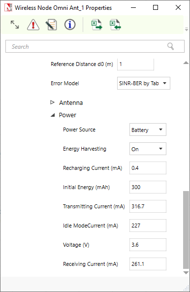
In NetSim, default energy model settings are as follows:
Transmitting current (mA): 316.7
Receiving current (mA): 261.1
Idle mode current (mA): 227
Voltage (V): 3.6
The power model is disabled by default. It can be enabled in physical layer of wireless node Omni Ant.
Click on a wireless node’s properties to open the right-side property panel, then navigate to Interface 1(Wireless) \(\triangleright\) Physical layer.
Mobility models in NetSim
The change in position of a user over time can be configured using mobility models. Such models are frequently used in simulation to evaluate the performance of mobile wireless systems. The mobility models available in NetSim are:
Random Walk Mobility Model
This is a simple mobility model based on random directions and speeds. In this mobility model, a mobile node moves from its current location to a new location by randomly choosing a direction. The speed can be set in the GUI. The calculation interval determines how often a new choice is made. For example, a 1s calculation interval means that a new position is chosen every 1s.
Random Waypoint Mobility Model
This model includes pause time between changes in direction and/or speed. A mobile node begins by staying in one location for a certain period of time (i.e., a pause time). Once this time expires, the mobile node chooses a random destination in the simulation area. The mobile node then travels toward the newly chosen destination at the selected speed. Upon arrival, the mobile node pauses for a specified PauseTime before starting the process again. Note that the movement calculation is done every Calculation Interval. Therefore, it is recommended to set the PauseTime as an integral multiple of Calculation Interval.
Group Mobility Model
This model describes the behavior of mobile nodes as they move together, i.e., the devices having common group id will move together.
Pedestrian Mobility Model
This model is applicable to each node (local parameter), and the configuration parameters are:
Pedestrian Max Speed (m/s) (Range: 0.0 to 10.0. Default: 3.0)
Pedestrian Min Speed (m/s) (Range: 0.0 to 10.0. Default: 1.0)
Pedestrian stop probability (Range: 0 to 1)
Pedestrian stop duration (s). (Range: 1 to 10000)
In this model it is assumed that the pedestrian stops at traffic lights. The stop probability represents the probability of encountering a traffic light. This is checked for every calculation interval. Once stopped, the pedestrian waits for a duration equal to stop duration for the light to turn green. A new direction is chosen randomly after every stop with \(\theta\) (angle between new direction and current direction) taking values of 0, 90, 180, 270. These \(\theta\) values represent the pedestrians continuing in the same direction, taking a left, making a U-turn, and taking a right, respectively.
A new speed is chosen randomly after event stop. \(\text{Min speed} \leq \text{Speed} \leq \text{Max speed}\)
The maximum number of stops and starts is 10.
File Based Mobility Model
In the File Based Mobility model, users can write their own custom mobility models and define the movement of the mobile users. The content should be per the NetSim Mobility File Format explained below. Users can also generate the mobility files using external tools like SUMO (Simulation of Urban Mobility), VanetMobiSim etc.
The NetSim Mobility File setting and format is explained below:
Step 1: Right click to open Properties as a new window of Wireless Node (MANET) or UE (LTE Networks). Then properties \(\triangleright\) Position Properties \(\triangleright\) Mobility model as File Based Mobility and click on Open Mobility file.
Step 2: Open the CSV file and write the node mobility in the format shown below.
<TIME IN SECONDS>,<DEVICE ID>,X,Y,Z
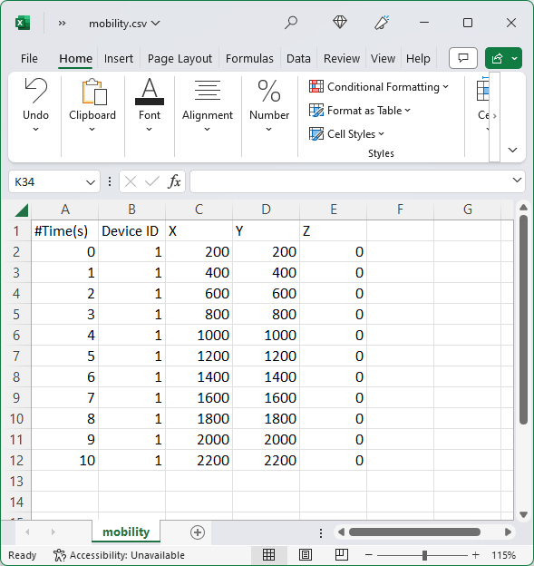
When using spreadsheet software commas (,) are included automatically between the entries in each column. When using text editors such as notepad, users will have to manually include comma (,) between each entry.

To write comments, use # tag
Specify the new location of the specific device at the specific time
Simulations with older input format in mobility.txt file (as shown below) will continue to be supported, in the absence of mobility.csv file.
$time <Time in seconds> ‘‘$node_(<NodeID - 1>) <X Coordinate> <Y Coordinate> <Z Coordinate>’’
Example: $time 1 ‘‘$node_(0) 400 400 0’’
A sample file-based mobility example is present at
<NetSim Installed Directory>\Docs\ Sample Configuration\ MANET.
It can have the coordinates of one node over time, followed by the coordinates of the next node over time and so on. However, for a given device, the entries in the file need to be in increasing order of time.
NetSim does not interpolate device mobility between two entries in the mobility file. This means that during the simulation the device “jumps” to the next point at that instant in time. Mobility is not “continuous” from one point to another over time. Continuous or fine-grained mobility can, however, be approximated by reducing the time interval between successive entries. Since Excel-based mobility files are supported, generating such fine-grained traces is straightforward.
Omni and sector (directional) antennas
NetSim MANET supports Omni and sector antennas. These antenna patterns are defined by gain values that vary as a function of direction in three dimensions. Thus, a transmitter’s antenna provides a gain value with respect to every other point in space. The same is true of a receiver’s antenna. For a given transmission, the gains of both the transmitter and receiver, with respect to each other, are considered.
Omni directional antennas have an isotropic pattern i.e., the gain in all directions is 0 dB. This makes them well-suited for scenarios where uniform coverage is required in all directions.
Sector antennas are modeled per the standard 2D parabolic antenna. The key characteristic of a sector antenna is its horizontal radiation pattern, which is designed to focus the signal in a specific direction. This directional pattern allows for targeted coverage, making sector antennas ideal for applications that require directed communication over a particular sector of space. The horizontal radiation pattern of a sector antenna is given by
\[\begin{equation} {A}_{E,H}\left(\varphi \right)=-\min\!\left(12\!\left(\frac{\varphi}{\varphi_{3\text{dB}}}\right)^{2},\;{A}_{m}\right) \end{equation}\]
where,
\({A}_{m}\) is the front to back ratio (i.e., the ratio of power gained between the front and rear of a directional antenna). This is a user input with a default setting of 30 dB.
\(\varphi\) is the angle formed between the direction of interest (i.e., the line connecting the transmitter and the receiver) and the antenna’s boresight direction (azimuth angle).
\(\varphi_{3\text{dB}}\) is the 3 dB, or half power, beam width of the antenna.
The sector antenna gain is given by the expression.
\[\begin{equation} {A}_{E}\left(\varphi,\theta\right)={G}_{E,\max}-\min\!\left\{-\left[{A}_{E,H}\left(\varphi\right)+{A}_{E,V}\left(\theta\right)\right],\;{A}_{m}\right\} \end{equation}\]
where,
\({A}_{E,V}\left(\theta\right)\) is currently 0 dB, and is a parameter reserved for future use to include the vertical radiation pattern of the antenna, and
\({G}_{E,\max}\) is the maximum directional gain of the radiation element (in dB) i.e., the gain along the antenna boresight; this parameter is a user input, and the default value is 8 dBi.
The boresight angle denotes the azimuthal direction of maximum gain, or the highest radiated power, and is a user input. This can vary from 0 to 360 degrees.
Angle in NetSim is defined to start at 0 from the positive X-axis. In the network scenario, if positive Y points downward, the angle increases on clockwise rotation from the positive X-axis. If positive Y points upward, the angle increases in an anti-clockwise direction from the positive X-axis. The unit for angle is degrees.
The gain computations for a transmitter-receiver pair are given below.

Let the transmitter be at \({X}_{1},{Y}_{1}\) and the receiver at \({X}_{2},{Y}_{2}\). Let \(\phi_{{T}_{X}}^{\text{boresight}}\) and \(\phi_{{R}_{X}}^{\text{boresight}}\) be the boresight azimuth angles of the transmitter and the receiver configured by the user through the GUI.
We know that, \[\begin{equation} \theta_{{T}_{X}-{R}_{X}}=\tan^{-1}\!\left(\frac{y_{2}-y_{1}}{x_{2}-x_{1}}\right) \end{equation}\]
and clearly, \[\begin{equation} \theta_{{R}_{X}-{T}_{X}}=\pi + \theta_{{T}_{X}-{R}_{X}} \end{equation}\]
\[\begin{equation} \phi_{{T}_{X}}=\phi_{{T}_{X}}^{\text{boresight}}-\theta_{{T}_{X}-{R}_{X}} \end{equation}\]
\[\begin{equation} \phi_{{R}_{X}}=\phi_{{R}_{X}}^{\text{boresight}}-\theta_{{R}_{X}-{T}_{X}} \end{equation}\]
The sign of \(\phi_{{T}_{X}}\) or \(\phi_{{R}_{X}}\) doesn’t matter since the square of the term is used in the gain calculations.
\[\begin{equation} {A}_{{T}_{X}}\left(\phi\right)=-\min\!\left[12\!\left(\frac{\phi_{{T}_{X}}}{\varphi_{3\text{dB}}}\right)^{2},\;A_{m}\right] \end{equation}\]
\[\begin{equation} {A}_{{R}_{X}}\left(\phi\right)=-\min\!\left[12\!\left(\frac{\phi_{{R}_{X}}}{\varphi_{3\text{dB}}}\right)^{2},\;A_{m}\right] \end{equation}\]
\[\begin{equation} T_{X}\;\text{Gain}={G}_{E,\max}-\min\!\left[-{A}_{{T}_{X}}\left(\phi\right),\;A_{m}\right] \end{equation}\]
\[\begin{equation} R_{X}\;\text{Gain}={G}_{E,\max}-\min\!\left[-{A}_{{R}_{X}}\left(\phi\right),\;A_{m}\right] \end{equation}\]
Enabling the radio measurements log allows for the visualization of transmit and receive antenna gains for each transmission.
Limitations
The vertical radiation pattern is not currently supported. Hence the horizontal radiation pattern is assumed to be valid for all values of the coordinate \(z\).
How are packet collisions modelled in NetSim
Packet Collision is a theoretical concept. In the real world, a packet is not a “physical” entity that can collide. Therefore, a “collision” is the interference of two radio waves (of the packets being sent).
In NetSim the collision model is as follows:
At the transmitter, when a packet is being transmitted, if the sum of received power from all other nodes is greater than the receiver sensitivity then that packet is marked as collided.
At the receiver, when a packet is being received, if the sum of the received power from all other nodes, except the node from where this packet is being transmitted, is greater than the receiver sensitivity then that packet is marked as collided.
There is also a special case where a single packet can be marked as collided as explained in Figure 3-3.
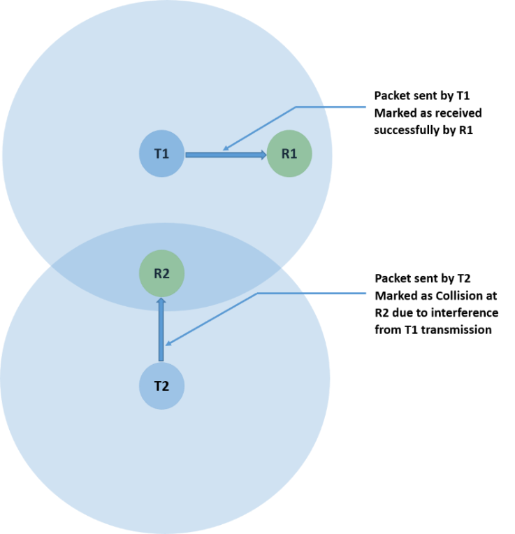
Where,
T1 and T2 are transmitters.
R1 and R2 are receivers.
How is packet error decided in NetSim
The way the packet error is decided is given as follows:
Compute Rx power at the receiver based on Tx Power, fewer losses due to Propagation. Propagation models cover HATA Urban, Sub Urban, COST 231 HATA, Indoor Home / Office, Factory, Lognormal, Free space. Apart from path loss, fading and shadowing can also be modeled.
Rx Power / (Background Noise + Interference noise) = SINR. Here Interference noise is due to other transmissions within the network.
Based on the SINR, BER is got from the respective modulation curve/table.
Based on the BER, the packet error rate is decided.
NetSim does not perform bitwise simulation since it would be too computationally intensive.
Broadcast in MANETs
In MANET, only neighbor (nodes within transmission range) broadcast is supported; multi-hop broadcast is not supported. This means that nodes that are 2-hops or more away will not receive the broadcast packets. The reason for not implementing a multi-hop broadcast is explained below.
The simplest form of broadcast in an ad hoc network is where a node transmits a broadcast packet, which is received by all neighboring nodes that are within transmission range. Upon receiving a broadcast packet, each node determines if it has transmitted the packet before. If not, then the packet is retransmitted. This process allows for a broadcast packet to be disseminated throughout the ad hoc network. The process terminates when all nodes have received and transmitted the packet being broadcast at least once.
This method of broadcasting is required given the dynamic nature of ad hoc networks, i.e., nodes move around, and neighbors may change as the broadcast is happening. Now, since all nodes participate in the broadcast, it causes flooding and hence suffers from the Broadcast Storm Problem. Flooding is extremely costly and leaves the network completely congested.
Special algorithms are required to alleviate the broadcast storm problem, and custom development is necessary to implement them.
Radio measurement log file and plots
NetSim IEEE 802.11 Radio Measurements log file records pathloss, shadowing loss, fading loss, received power, transmitted power, SNR, and BER. This log can be enabled by clicking on configure reports in top ribbon \(\triangleright\) Plots \(\triangleright\) Select IEEE 802.11 Radio Measurements log under Network Logs as shown below

The IEEE802.11 Radio Measurements log.csv file will contain the following information:
Time in Milliseconds
Transmitter Name
Receiver Name
Distance between the Transmitter and the Receiver in meters
Packet ID
Packet Type
Control Packet Type
Transmitter Power in dBm
Pathloss in dB
Shadowing Loss in dB
Fading Loss in dB
Total Loss in dB
Transmitter Antenna Gain in dB
Receiver Antenna Gain in dB
Received Power in dBm
Interference in dBm
SNR in dB
SINR in dB
BER
NSS (Number of Spatial Streams)
MCS Index
The log file can be accessed from the Simulations Results Window under the log as shown below.


NetSim plots
NetSim also provides energy and Wi-Fi radio measurement plots for MANET. Enabling the plots is explained in the section 2.6. Here is the plot showing the transmit energy vs. time for an AODV scenario with five nodes.

The Wi-Fi Radio measurement plots are shown in featured example in section 4.8.