Featured Examples
Sample configuration files for all networks are available in Examples Menu in NetSim Home Screen. These files provide examples on how NetSim can be used – the parameters that can be changed and the typical effect it has on performance.
AODV Routing
The Ad hoc On Demand Distance Vector Routing (AODV) protocol defines 3 message types:
Route Requests (RREQs): RREQ messages are used to initiate the route-finding process.
Route Replies (RREPs): RREP messages are used to finalize the routes.
Route Errors (RERRs): RERR messages are used to notify the network of a link breakage in an active route.
The route discovery process involves ROUTE REQUEST (RREQ) and ROUTE REPLY (RREP) packets. The source node initiates the route discovery process using RREQ packets. The generated route request is forwarded to the neighbors of the source node and this process is repeated till it reaches the destination. On receiving an RREQ packet, an intermediate node with route to destination or the destination node generates an RREP containing the number of hops required to reach the destination. All intermediate nodes that participate in relaying this reply to the source node create a forward route to destination.
RERR message processing is initiated when Node detects a link break for the next hop of an active route or receives a data packet destined for a node for which it has no (active) route.
Open NetSim and Select Examples\(\rightarrow\)Mobile Ad hoc Networks\(\rightarrow\)MANET AODV then click on the tile in the middle panel to load the example as shown in below screenshot Figure 4-1.

The following network diagram illustrates, what the NetSim UI displays when you open the example configuration file see Figure 4-2.
Network Settings
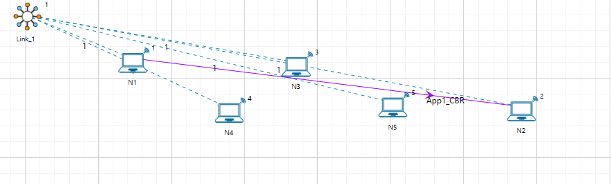
A network scenario is designed in NetSim GUI, consisting of 5 wireless nodes omni ants, named N1, N2, N3, N4, and N5, and one link in the “Standard MANET” of the “Mobile Ad hoc Network” library.
In the general properties of N3, Wireshark Capture is set to Online. To configure any properties in the nodes, click on the node, expand the property panel on the right side, and change the properties as mentioned in the steps.
In the position properties, set the mobility model as No-Mobility for all devices present in the GUI.
The Medium Access Protocol is set to DCF in Interface 1(Wireless)\(\rightarrow\) Datalink layer of all the devices.
Click on link and expand property panel on the right, and set the Channel Characteristics: Path loss only; Path loss model: Log Distance; Path loss exponent: 3.1.
The routing protocol in the network layer is set to AODV for all nodes. As this is a global property, changing it on one node will affect all nodes.
Packet trace is enabled by clicking on the configure report tab, allowing us to track the route that the packets have taken to reach the destination based on AODV.
Configure the CBR application between two nodes by clicking on the set traffic tab from the ribbon at the top, selecting N1 as the source and N2 as the destination. Click on the created application and set the transport protocol to UDP, keeping the other properties as default.
Run simulation for 10 seconds.
Open packet trace from simulation results window.
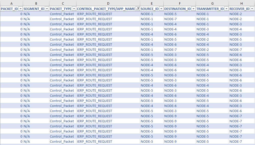
The packet flow can be observed by filtering Control Packet Type/App Name to AODV RREQ, AODV RREP and AODV RREP (Hello) as shown below.
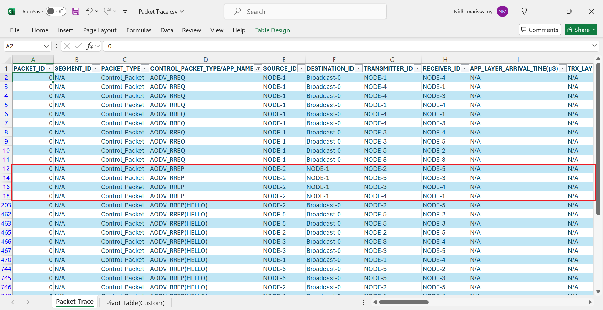
Source Node 1 initiates route discovery process using RREQ packets. The generated route request is broadcast to the neighbors of the source node i.e. Node 4.
Node 4 broadcasts the RREQ packet to its neighboring nodes i.e., Node 3, Node 1 since Node 4 does not have a route to destination Node 2.
Similarly, Node3 broadcasts the RREQ packet to Node 5 and Node 4.
Node 5 broadcasts to Node 2 and Node 3.
On receiving a RREQ packet, the Destination Node 2 generates a RREP packet and transmits to Node 5, Node 2 \(\rightarrow\) Node 5, Node 5 \(\rightarrow\) Node 3, Node 3 \(\rightarrow\) Node 4, and Node 4 \(\rightarrow\) Node 1.
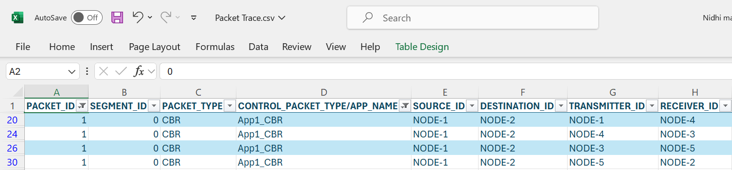
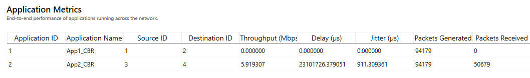
After receiving the RREP, the Source Node 1 starts sending Data packets to Node 2 (Node 1 \(\rightarrow\) Node 4 \(\rightarrow\) Node 3 \(\rightarrow\) Node 5 \(\rightarrow\) Node 2). To observe the same, filter the CONTROL PACKET TYPE/APP NAME to APP1_CBR and PACKET ID to 1 in packet trace.
In Wireshark, filter AODV packets and select the RREQ packets and expand Ad hoc on-demand distance vector protocol to view the above-mentioned fields of RREQ as shown in Figure 4-4.

Open Wireshark, filter AODV packets and select the RREP packets and expand Ad hoc on-demand distance vector protocol to view the above-mentioned fields of RREP as shown in Figure 4-5.

ZRP-IARP
Open NetSim and select Examples\(\rightarrow\)Mobile Ad hoc Networks\(\rightarrow\)ZRP IARP then click on the tile in the middle panel to load the example as shown in below screenshot Figure 4-6.
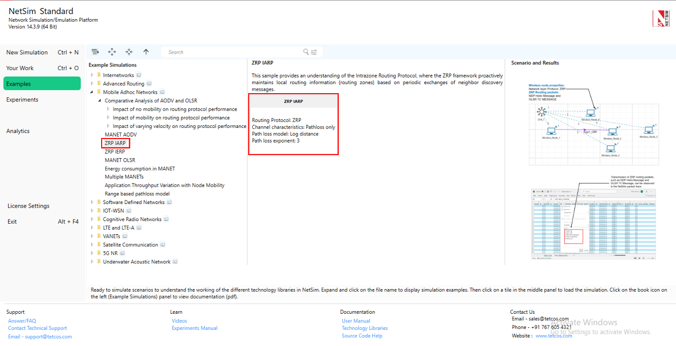
The following network diagram illustrates what the NetSim UI displays when you open the example configuration file see Figure 4-7.

Network Settings
Set grid length as 600m\(\times\)300m from grid setting property panel on the right. This needs to be done before any device is placed on the grid.
A network scenario is designed in NetSim GUI consisting of 5 wireless nodes and one ad-hoc link in the “Standard MANET” module of MANET Network library.
To configure any properties in the nodes, click on the node, expand the property panel on the right side, and change the properties as mentioned in the below steps.
In the position properties set mobility model as no mobility for all devices present in GUI.
The Medium access protocol was set to DCF in Interface 1(wireless)\(\rightarrow\) Datalink layer of all Wireless nodes.
The routing protocol in the network layer is set to ZRP for all nodes. As this is a global property, changing it on one node will affect all nodes.
Click on link and expand property panel on the right and set the channel characteristics: path loss only, path loss model: log distance, path loss exponent: 3 under medium property.
Configure CBR application from set traffic tab in ribbon on the top between wireless node 1 to wireless node 2, click on the created application, expand the property panel on the right and set transport protocol to UDP.
Enable packet trace from configure reports tab in ribbon on the top.
Run simulation for 10 seconds.
Output
Open Packet trace from simulation results window and observe Control Packet Type/App Name.

Users can see only NDP Hello Message and OLSR TC MESSAGE since the destination node is within the zone. The ZRP framework proactively maintains local routing information (routing zones) based on periodic exchanges of neighbor discovery messages.
ZRP-IERP
Open NetSim and Select Examples \(\rightarrow\) Mobile Ad hoc Networks \(\rightarrow\) ZRP IERP then click on the tile in the middle panel to load the example as shown in below screenshot Figure 4-9.

The following network diagram illustrates what the NetSim UI displays when you open the example configuration file see Figure 4-10.

Network Settings
Set grid length as 600m\(\times\)300m from grid setting property panel on the right. This needs to be done before any device is placed on the grid.
A network scenario is designed in NetSim GUI consisting of 12 wireless nodes and one ad-hoc link in the “Standard MANET” of MANET Network library.
To configure any properties in the nodes, click on the node, expand the property panel on the right side, and change the properties as mentioned in the below steps.
In the position properties set mobility model as No mobility for all devices present in GUI.
The medium access protocol was set to DCF in Interface 1(wireless)\(\rightarrow\) Datalink layer of all wireless nodes.
The routing protocol in the network layer is set to ZRP for all nodes. As this is a global property, changing it on one node will affect all nodes.
Click on link and open property panel on the right and set the Channel characteristics: Log distance, Path loss exponent: 2.9.
Configure CBR application from wireless nodes 1 to wireless nodes 12 by clicking on set traffic tab in ribbon on the top. Click on the created application and set the transport protocol to UDP, keeping the other properties as default.
Enable Packet Trace from configure reports tab in the ribbon on the top.
Run simulation for 10 seconds.
Output
Open packet trace and filter Control Packet Type/App Name to IERP route request. In the below packet trace, node-1 is sending IERP route request packets to its peripheral nodes 2 and 3 since the destination is not present in node1’s zone. Similarly, Node 2 transmits IERP route request packets to node 5 and 7 and node 3 transmits to node 4. To observe the IERP route request flow from the respective nodes filter the Transmitter Id to Node 1, Node 2 and Node 3 alone.
Node 7 generates an IERP Route Reply packet in response to the IERP Route Request since the destination node, Node 12, is present in the Node 7 zone. IERP Route Reply packet routes through Node 7 \(\rightarrow\) Node 2 and Node 2 \(\rightarrow\) Node 1. And the data packet routes through Node 1 \(\rightarrow\) Node 2, Node 2 \(\rightarrow\) Node 7, Node 7 \(\rightarrow\) Node 9 and Node 9 \(\rightarrow\) Node 12.

MANET-OLSR
Part-1: MPR Table Formation in NetSim
Introduction
In OLSR, only a subset of preselected nodes called MPR (Multi-Point Relays) are used to perform topological advertisements. Control messages (containing e.g. routing information) are broadcast and forwarded only by MPRs. This leads to a reduction in the number of transmitter nodes, in the overhead and in useless receptions of messages on nodes. The well-known storm problem due to broadcasting is avoided.
Creation of MPRs in OLSR
Neighbor Discovery
Each node in the OLSR network periodically broadcasts HELLO messages to its immediate neighbors. These messages contain information about the node itself and its direct neighbors (1-hop neighbors).
From these HELLO messages, a node learns about its 1-hop and 2-hop neighbors (the neighbors of its neighbors).
MPR Selection
Goal: The primary goal of selecting MPRs is to ensure that all 2-hop neighbors of a node can be reached through at least one of its MPRs.
A node selects a subset of its 1-hop neighbors as MPRs in such a way that these MPRs can cover all of its 2-hop neighbors. This means that every 2-hop neighbor must be reachable via at least one selected MPR.
The selection of MPRs is done based on degree of connectivity – nodes with a larger number of 2-hop neighbors might be preferred to cover more ground with fewer MPRs.
Route Calculation Using MPRs
Only the nodes selected as MPRs are responsible for forwarding control messages like Topology Control (TC) messages. This significantly reduces the number of transmissions, leading to less network overhead.
When a node needs to broadcast a TC message, it only forwards it to its MPRs, which in turn continue the broadcast, ensuring that the entire network receives the update.

In the first step, a node, node U (the green node in the diagram), selects relays from its one-hop neighbors (N1). These relays, referred to as MPR1 nodes (highlighted in blue), ensure that all isolated nodes in its two-hop neighborhood (N2), shown in red, are reachable. For instance, node T is considered an isolated node that can only connect to node U through node H. Therefore, node H is elected as an MPR in this step, ensuring node T can reach U in two hops.
In the second step, node U focuses on covering any remaining nodes in its two-hop neighborhood that were not connected by the initial MPR selection. It considers nodes in N2 that remain uncovered, as well as one-hop neighbors not chosen in the first step, like nodes B, F, E, and D. Node U then selects additional MPRs based on their connectivity to maximize coverage. For example, node E is chosen because it can cover multiple nodes in N2 that would otherwise remain isolated. The algorithm concludes when all nodes within two hops of node U are connected, forming an efficient routing set, represented as MPR(U) = {C, E, I, H, G} in the diagram. This process ensures optimal coverage while minimizing redundant transmissions.
3D Network Topology
In the network topology illustrated in Figure 4-13, connecting lines indicate that two nodes are within communication range of each other, while the absence of a line signifies that the nodes are out of range. The specific distance requirements between nodes create a set of spatial constraints that cannot be satisfied when nodes are arranged only in the X-Y plane. To resolve this geometric limitation, the nodes are positioned in three-dimensional space, utilizing the Z-axis to achieve the required connectivity pattern. The coordinates of the nodes are given in the table below.
| Node ID | X | Y | Z |
|---|---|---|---|
| 1 (U) | 500.00 | 250.00 | 150 |
| 2 | 500.00 | 150.00 | 230 |
| 3 | 571.00 | 179.00 | 70 |
| 4 | 600.00 | 250.00 | 230 |
| 5 | 571.00 | 321.00 | 70 |
| 6 | 500.00 | 350.00 | 230 |
| 7 | 429.00 | 321.00 | 70 |
| 8 | 399.83 | 249.15 | 230 |
| 9 | 429.00 | 179.00 | 70 |
| 10 | 394.06 | 105.73 | 0 |
| 11 | 382.76 | 113.09 | 130 |
| 12 | 571.78 | 97.90 | 130 |
| 13 | 614.60 | 118.89 | 0 |
| 14 | 624.00 | 289.00 | 160 |
| 15 | 564.00 | 263.00 | 0 |
| 16 | 545.27 | 396.84 | 170 |
| 17 | 455.00 | 437.00 | 65 |
| 18 | 393.35 | 300.00 | 0 |
| 19 | 352.03 | 339.62 | 150 |
| 20 | 330.36 | 252.03 | 300 |
A 3D view of the topology is shown in Figure 4-14 below.

Network Setup
Open NetSim and Select Examples \(\triangleright\) Mobile Ad hoc Networks \(\triangleright\) MANET-OLSR then click on the tile in the middle panel to load the example as shown in below.

The following steps were carried out to generate this scenario:
Set grid length as 1000 \(\times\) 500 from grid setting property panel on the right. This needs to be done before any device is placed on the grid.
Create a scenario with 20 Nodes as shown in Figure 4-13.
Click on wireless node, expand the property panel on right and go to Position layer \(\triangleright\) set Mobility model to No mobility in all nodes.
Set the Routing protocol to OLSR in Network layer of wireless nodes. As this is a global property, changing it on one node will affect all nodes.
Click on the link, expand link property on right and set the channel characteristics to pathloss and pathloss model as Range based, with range as 130m.
Enable OLSR Neighbor and MPR log by clicking on configure reports tab and plots as shown below.

Enabling OLSR Neighbor and MPR log Run the simulation for 50 seconds.
Results and Analysis
In the Results dashboard, click on logs tab and open OLSR_MPR_Log.csv file.
Filter the device name column to U.

Initially, U starts with a single MPR node, “E,” at 1598.32 ms. Over time, more nodes are added to the MPR list (e.g., “C”, “H”, “I”, “G”), with some nodes being dropped or rearranged.
We finally get the set of MPR nodes as “C; I; G; H; E”.
Part-2: NDP and TC Messages in OLSR
Introduction
OLSR Hello Messages (NDP)
The OLSR Hello messages, part of the Neighbor Discovery Protocol (NDP), are exchanged between directly connected nodes. They enable each node to detect its one-hop and two-hop neighbors. These messages are used to establish and maintain neighbor relations, which are necessary for building an updated and accurate network topology. Hello messages include information about link status and the willingness of a node to participate in forwarding traffic for its neighbors. This process helps in selecting Multipoint Relays (MPRs), which minimize the number of transmissions required for routing updates.
OLSR TC Messages

Network Setup
Consider the same scenario as Part -1.
Click on wireless node U, expand property panel on right and go to General Layer Set Wireshark Capture to Online.
Go to Configure Reports tab \(\rightarrow\) Enable Packet trace.
Run the simulation for 50 seconds.
Results and Analysis
Wireshark is generated during the simulation of network.
The periodic exchange of Hello messages in OLSR dynamically updates the MPR (Multi-Point Relay) list of a device. You can observe this in the OLSR_MPR_Log.csv by filtering the Device Name column to “U.”
Neighbor Discovery Process (NDP) or Hello Messages
See Figure 4-20.
Initial MPR Selection: At 1598.32 ms, the device starts with a single MPR node, “E.” This means “E” was initially the best choice for relaying messages.
MPR List Evolution: Over time, more nodes like “C,” “H,” “I,” and “G” are added to the list. This indicates the device is adapting to network changes, selecting new relays as network conditions evolve.
Dynamic Changes: Nodes are added or removed from the MPR list based on their current efficiency in relaying messages, reflecting ongoing adjustments to the network topology.
Multiple MPR Nodes: We finally get the set of MPR nodes as “C; I; G; H; E”.

Topology Control (TC) Messages
TC (Topology Control) messages are periodically exchanged to inform nodes about the network’s topology. Each node updates its routing table based on the information in these messages, which include details about MPRs (Multi-Point Relays) and their connections.
When a node receives a TC message, it uses the link information to add or adjust routes in its table, ensuring it always has the most efficient paths to other nodes. This dynamic updating keeps the network adaptive to changes, such as new routes or broken links.


The routing table shown in Figure 4-22 reflects these updates, displaying the optimal routes formed from the latest TC message exchanges.
How often are NDP Hello Messages and TC Messages exchanged in the Network
Open Packet trace from simulation results window and filter Control Packet Type/App Name to NDP HELLO MESSAGE, Source ID to Node-1. All the nodes in the network exchange the NDP HELLO MESSAGEs periodically (for every 2 seconds—check NETWORK LAYER ARRIVAL TIME column) to detect the neighbors. In the below screenshot, Node-1 is broadcasting NDP HELLO MESSAGES to its neighbors 2, 3, 4, 5, 6, 7, 8 and 9 for every 2 seconds as shown below.

You can observe in the packet trace that hello packets are exchanged every 1.7 seconds. This is obtained from
\(\text{Actual Message Interval} = \text{Message Interval} - \text{Jitter}\)
This is applicable for TC messages as well.
Now filter Control Packet Type/App Name to OLSR TC Message, Source Id and Transmitter Id to Node-1. All nodes in the network, broadcasts Topology control (TC) messages (for every 5 seconds—check Network layer arrival time column) in order to build the topology information base. In the below screenshot, node-1 is broadcasting OLSR TC Message to its neighbors 2, 3, 4, 5, 6, 7, 8 and 9 for every 5 seconds as shown below.

Comparative analysis of AODV and OLSR in static and mobility scenarios
Introduction
Mobile Ad hoc Networks (MANETs) are self-organizing wireless networks that operate without a fixed infrastructure. The dynamic and distributed nature of MANETs introduces challenges for routing protocols, particularly in handling topology changes and maintaining efficiency under varying traffic loads. Routing protocols for MANETs are broadly categorized into reactive and proactive approaches, each with distinct mechanisms and trade-offs.
Ad-hoc On-Demand Distance Vector (AODV): AODV is a reactive routing protocol that establishes routes only when needed. As described by Clausen et al., AODV initiates route discovery by broadcasting route request packets, followed by unicast replies for discovered routes. This approach reduces control overhead in static or low-traffic networks. However, frequent route rediscoveries caused by mobility or high traffic densities can increase overhead.
Optimized Link State Routing (OLSR): OLSR is a proactive protocol that maintains routing tables for all nodes in the network at all times. Clausen et al. highlight OLSR’s use of Multipoint Relays (MPRs) to optimize control traffic by reducing redundant retransmissions during periodic updates. While OLSR ensures immediate route availability, it generates constant control traffic regardless of traffic flow or mobility.
This example evaluates and compares the performance of AODV and OLSR under three scenarios:
No mobility: Nodes remain stationary throughout the simulation.
With mobility: Nodes follow a random walk mobility model, but with a fixed speed.
Varying velocity: Nodes move at speeds ranging from 0 m/s to 100 m/s.

We analyze which protocol is more resource-efficient under different network conditions, focusing on control traffic overhead, which refers to the additional network traffic generated by routing protocols during activities such as route discovery, updates, and maintenance. Since excessive control traffic can degrade performance in MANETs by consuming the already limited bandwidth, minimizing this overhead is crucial for efficient network operation. By comparing AODV and OLSR, this study provides insights into their suitability for specific scenarios, helping users make appropriate decisions based on trade-offs between scalability, bandwidth utilization, and control overhead.
Simulation Setup
Network Configuration
These settings have been pre-configured in the simulation environment.
| Simulation Parameters | Value |
|---|---|
| Environment size | 10000 \(\times\) 5000 |
| Mobility model | No mobility/Random walk |
| Velocity | 10 m/s (only for Random walk) |
| Calculation Interval | 2 second (only for Random walk) |
| Routing protocol | AODV/OLSR |
| MAC protocol | 802.11 b |
| Transmission range | 1700 m |
Setting transmission range in NetSim: Click on the link connecting the nodes and open the link properties by navigating to the medium property in the link properties panel (RHS).
Set channel characteristics to pathloss, choose Range based for the pathloss model, and enter 1700 m in the Range (m) field.

Configuring transmission range in NetSim link properties. Enable packet trace from the configure reports tab in ribbon on top.
Run the simulation for 50 seconds.
Scenario Setup
For both AODV and OLSR, we simulate 30 cases with varying numbers of applications. Each case increases the number of applications by one, starting from a single application in Case 1 and going up to 30 applications in Case 30.
Repetition of Simulations
To reduce the impact of randomness, each scenario (AODV and OLSR) is repeated with three sets of simulations:
Set 1: Initial set of source-destination pairs.
Set 2: Second set of source-destination pairs.
Set 3: Third set of source-destination pairs.
The final results are the averaged control traffic overhead across these three sets.
In the NetSim GUI, we provide configuration files for three cases: mobility, No-mobility, and velocity. The dataset includes:
Mobility Cases:
Set 1: 30 cases of AODV and OLSR.
No-Mobility Cases:
Set 1: 30 cases of AODV and OLSR.
Velocity Cases:
Set 1: 10 cases of AODV and OLSR across varying velocities.
The complete set of configuration files is available for download: GitHub Zip folder download link: https://github.com/NetSim-TETCOS/Comparative-analysis-of-AODV-and-OLSR-v14.4/archive/refs/heads/main.zip
Click on the link above to download the comparative analysis examples.
Extract the zip folder. The extracted project folder consists of case files for mobility, No-mobility, and velocity cases.
Instructions for importing the workspace are provided in section 4.9.2 of the NetSim user manual.
Steps for Control Traffic Overhead Calculation
Running the Simulation
Open NetSim and Select Examples\(\rightarrow\) Mobile Ad hoc Networks \(\rightarrow\) Comparative Study of AODV and OLSR

For this example, Open the No-mobility case-10 scenario (e.g., No-mobility case \(\triangleright\) Set-1 \(\triangleright\) AODV \(\triangleright\) case-10), which is configured with 10 applications.
Run the simulation for 50 seconds.
Accessing the Packet Trace
After each simulation is completed, open the packet trace file generated from the result dashboard.

This file contains detailed logs for each packet transmitted in the network.
Filtering Control Packets for AODV
In this step, we filter AODV control packets specifically to calculate the control traffic overhead accurately:

Filtering by Control Packet Type: We select only rows where Control Packet Type/App Name specifies AODV. This isolates the AODV-specific control traffic data.
Removing Duplicate Entries
Broadcast control packets, used by AODV/OLSR during route discovery, are transmitted to all neighbouring nodes within range. In all these cases the same packet is received and logged by multiple nodes. Since each neighbor logs the packet, the same packet(s) appears multiple times in the data, however the packet(s) was transmitted only once by the sender.

For example, a packet sent by Node-9 may be received by multiple nodes (Node-2, Node-5, etc.) at the same Phy layer start time(\(\mu\)S).
By keeping only unique entries based on Packet Id and Phy layer start time(\(\mu\)S), we avoid counting the same packet multiple times, which would otherwise inflate the overhead.
Steps to remove Duplicate packet entries.
Go to Data \(\triangleright\) Remove Duplicates in your spreadsheet software.
In the Remove Duplicates dialog:

Unselect all columns.
Select only the columns Packet Id and Phy layer start time(\(\mu\)S).
This will remove duplicate AODV control packets based on packet ID and start time.
Calculating the Control Traffic Overhead
In the filtered data, locate the Phy layer pay load(Bytes) column.

Finally, we calculate the sum of Phy layer payload (Bytes) for the unique entries. This gives the actual control traffic overhead for AODV, ensuring an accurate representation of the protocol’s overhead without duplicate broadcasts.
Record this sum as the Control traffic overhead for the current case of AODV.
Repeating for OLSR
Configure the network layer protocol to OLSR instead of AODV.
Follow steps from 4.5.5.3 to 4.5.5.5 to calculate the control traffic overhead for each case of OLSR.
In step 4.5.5.3, filter for OLSR packets in the Control Packet Type/App Name column.

Here just filter NDP Hello Message and OLSR TC Message
Repeat steps 4.5.5.1 to 4.5.5.5 for each case (Case 1 to Case 30) of AODV and OLSR.
Record the overhead values.
Averaging Across Sets
Calculate the control traffic overhead for Set 1.
Repeat the calculations for Set 2 and Set 3.
Average the control traffic overhead values from sets 1, 2, and 3 to obtain the final control traffic overhead for each case.
We have used the same method to get the results for Mobility case also.
Results and Discussion
No-Mobility cases
The results for the No-mobility case of these three sets are as follows:
| Set 1 (Ctrl Traffic OH) | Set 2 (Ctrl Traffic OH) | Set 3 (Ctrl Traffic OH) | Average | |||||
|---|---|---|---|---|---|---|---|---|
| 2-3(lr)4-5(lr)6-7(lr)8-9 No. of Traffic flows | AODV(B) | OLSR(B) | AODV(B) | OLSR(B) | AODV(B) | OLSR(B) | AODV(B) | OLSR(B) |
| 2-3(lr)4-5(lr)6-7(lr)8-9 No. of Traffic flows | AODV(B) | OLSR(B) | AODV(B) | OLSR(B) | AODV(B) | OLSR(B) | AODV(B) | OLSR(B) |
| 25408 | 318344 | 26176 | 276420 | 25424 | 319832 | 25669 | 304865 | |
| 2 | 26520 | 276716 | 26972 | 275840 | 28160 | 290088 | 27217 | 280881 |
| 3 | 27896 | 268724 | 26972 | 275644 | 30924 | 288556 | 28597 | 277641 |
| 4 | 27348 | 268388 | 27588 | 276344 | 30228 | 280944 | 28388 | 275225 |
| 5 | 28204 | 276944 | 29308 | 288980 | 32320 | 282740 | 29944 | 282888 |
| 6 | 31052 | 283036 | 30324 | 290512 | 32284 | 280896 | 31220 | 284815 |
| 7 | 30848 | 274488 | 32180 | 269492 | 29772 | 303224 | 30933 | 282401 |
| 8 | 32584 | 272836 | 32956 | 302984 | 31596 | 295732 | 32379 | 290517 |
| 9 | 34360 | 275576 | 33108 | 359952 | 35016 | 281708 | 34161 | 305745 |
| 10 | 33616 | 274608 | 36252 | 323924 | 32548 | 308024 | 34139 | 302185 |
| 11 | 36476 | 287084 | 90788 | 367112 | 34268 | 296432 | 53844 | 316876 |
| 12 | 38444 | 280592 | 44644 | 322924 | 38084 | 281432 | 40391 | 294983 |
| 13 | 38376 | 299092 | 38940 | 314984 | 39712 | 290436 | 39009 | 301504 |
| 14 | 49996 | 271380 | 48136 | 350124 | 35320 | 313092 | 44484 | 311532 |
| 15 | 48060 | 370212 | 48212 | 321040 | 42052 | 291232 | 46108 | 327495 |
| 16 | 46852 | 311964 | 59984 | 334160 | 42356 | 324404 | 49731 | 323509 |
| 17 | 51872 | 299616 | 91728 | 337736 | 38832 | 345300 | 60811 | 327551 |
| 18 | 51668 | 299444 | 91840 | 316672 | 57864 | 319764 | 67124 | 311960 |
| 19 | 52184 | 298344 | 69356 | 311544 | 47020 | 334884 | 56187 | 314924 |
| 20 | 52824 | 284920 | 75636 | 305984 | 78740 | 292116 | 69067 | 294340 |
| 21 | 75048 | 328816 | 78500 | 347088 | 542100 | 327960 | 231883 | 334621 |
| 22 | 79456 | 263516 | 455780 | 337488 | 59932 | 284844 | 198389 | 295283 |
| 23 | 89332 | 268588 | 2380728 | 339088 | 79424 | 311472 | 849828 | 306383 |
| 24 | 85116 | 289088 | 2915412 | 392956 | 126364 | 280832 | 1042297 | 320959 |
| 25 | 82756 | 263900 | 1369760 | 351040 | 1989620 | 339460 | 1147379 | 318133 |
| 26 | 2083272 | 320484 | 2360080 | 389672 | 1786548 | 317028 | 2076633 | 342395 |
| 27 | 1385988 | 298800 | 3691028 | 322368 | 2056808 | 351144 | 2377941 | 324104 |
| 28 | 2168944 | 334812 | 2564324 | 309036 | 3477228 | 302272 | 2736832 | 315373 |
| 29 | 1064636 | 330868 | 3782316 | 329388 | 3560280 | 272748 | 2802411 | 311001 |
| 30 | 2556544 | 356724 | 4280888 | 392928 | 2235200 | 309268 | 3024211 | 352973 |
This table presents the control overhead data for 30 traffic flows, averaged across three simulation sets (Set 1, Set 2, and Set 3) with unique source-destination pairs. The averaging process reduces randomness and ensures a more accurate comparison for both the no mobility and mobility scenarios.
Plot:

Mobility cases
The results for the Mobility case of these three sets are as follows:
| Set 1 (Ctrl Traffic OH) | Set 2 (Ctrl Traffic OH) | Set 3 (Ctrl Traffic OH) | Average | |||||
|---|---|---|---|---|---|---|---|---|
| 2-3(lr)4-5(lr)6-7(lr)8-9 No. of flows | AODV(B) | OLSR(B) | AODV(B) | OLSR(B) | AODV(B) | OLSR(B) | AODV(B) | OLSR(B) |
| 2-3(lr)4-5(lr)6-7(lr)8-9 No. of flows | AODV(B) | OLSR(B) | AODV(B) | OLSR(B) | AODV(B) | OLSR(B) | AODV(B) | OLSR(B) |
| 25468 | 412680 | 25468 | 412680 | 27564 | 352936 | 26167 | 392765 | |
| 2 | 26100 | 314384 | 27732 | 490148 | 27568 | 384508 | 27133 | 396347 |
| 3 | 28284 | 297648 | 27816 | 470056 | 27684 | 419320 | 27928 | 395675 |
| 4 | 28608 | 383552 | 30364 | 304816 | 31836 | 478392 | 30269 | 388920 |
| 5 | 29212 | 414160 | 31396 | 316880 | 30684 | 372984 | 30431 | 368008 |
| 6 | 31328 | 443772 | 32928 | 456948 | 31876 | 434908 | 32044 | 445209 |
| 7 | 32536 | 350376 | 35684 | 465236 | 32808 | 493136 | 33676 | 436249 |
| 8 | 32752 | 370728 | 31396 | 373828 | 32808 | 433900 | 32319 | 392819 |
| 9 | 35044 | 322424 | 31636 | 350124 | 33824 | 398684 | 33501 | 357077 |
| 10 | 34068 | 373596 | 34280 | 401796 | 36032 | 308160 | 34793 | 361184 |
| 11 | 39036 | 376044 | 37544 | 349312 | 37248 | 343312 | 37943 | 356223 |
| 12 | 36660 | 354536 | 39668 | 458356 | 39644 | 394156 | 38657 | 402349 |
| 13 | 37036 | 315992 | 48180 | 369068 | 44104 | 416508 | 43107 | 367189 |
| 14 | 47028 | 443904 | 42636 | 449600 | 53084 | 395444 | 47583 | 429649 |
| 15 | 50748 | 408052 | 50012 | 341944 | 355392 | 354320 | 152051 | 368105 |
| 16 | 59056 | 420716 | 1355420 | 448332 | 60640 | 414000 | 491705 | 427683 |
| 17 | 62776 | 423056 | 183964 | 506256 | 62644 | 337688 | 103128 | 422333 |
| 18 | 60436 | 459968 | 71752 | 335768 | 52292 | 442308 | 61493 | 412681 |
| 19 | 126680 | 377748 | 60120 | 261748 | 77252 | 431580 | 88017 | 357025 |
| 20 | 63424 | 349852 | 110380 | 331340 | 72000 | 392752 | 81935 | 357981 |
| 21 | 98604 | 396896 | 2194176 | 363072 | 99292 | 359712 | 797357 | 373227 |
| 22 | 743344 | 483432 | 3502212 | 442140 | 76796 | 522720 | 1440784 | 482764 |
| 23 | 3766092 | 419096 | 2906148 | 487928 | 100112 | 366276 | 2257451 | 424433 |
| 24 | 511088 | 363200 | 3594464 | 491992 | 1515364 | 390620 | 1873639 | 415271 |
| 25 | 3115056 | 436116 | 2297716 | 389652 | 1916896 | 397768 | 2443223 | 407845 |
| 26 | 2756380 | 384908 | 2900080 | 429592 | 2454956 | 453184 | 2703805 | 422561 |
| 27 | 1902272 | 361012 | 4675832 | 471316 | 2272428 | 424092 | 2950177 | 418807 |
| 28 | 1716844 | 438220 | 4297136 | 442520 | 2845088 | 407636 | 2953023 | 429459 |
| 29 | 2546728 | 328956 | 3420656 | 319520 | 2909900 | 425556 | 2959095 | 358011 |
| 30 | 776816 | 417396 | 3729096 | 372632 | 3061636 | 399436 | 2522516 | 396488 |
Plot:

Discussion
AODV Control Overhead
In both no-mobility and mobility scenarios, AODV initially performs better for approximately the first 1–18 traffic flows, maintaining lower control traffic overhead compared to OLSR. This is due to its reactive nature, where route discovery is triggered only when required, minimizing unnecessary control packets in low-traffic conditions.
However, beyond 1–18 traffic flows, the control overhead for AODV increases drastically in both scenarios. This sharp rise is due to the additional route discovery processes triggered by increasing traffic flows. In mobility scenarios, this increase is further amplified by frequent route rediscoveries caused by dynamic topology changes.
OLSR Control Overhead
OLSR exhibits consistent control overhead across all traffic flows in both no-mobility and mobility scenarios. Its proactive nature, characterized by periodic routing updates, ensures stable performance regardless of traffic flow density or mobility.
While OLSR’s overhead is slightly higher than AODV’s for fewer than 10 traffic flows, it becomes the more efficient protocol as traffic density increases, due to its predictable and scalable performance.
Insights
The results highlight the following key observations:
Low traffic loads: AODV has an advantage in sparse traffic scenarios (up to 10 traffic flows), where its reactive mechanism minimizes unnecessary control overhead.
High traffic loads: OLSR exhibits better scalability and predictability for networks with moderate to high traffic densities.
Impact of Mobility: While mobility introduces additional control traffic for AODV due to frequent route rediscoveries, the overall trend remains similar to the no-mobility scenario, with traffic flow density being the dominant factor.
Impact of Varying Velocity on Routing Protocol Performance
In MANETs, the velocity of nodes significantly influences the dynamics of the network topology. As nodes move faster, link breakages and re-establishments occur more frequently, posing challenges for routing protocols.
Scenario Setup
These settings have been pre-configured in the simulation environment.
| Simulation Parameters | Value |
|---|---|
| Environment Size | 10000 \(\times\) 5000 |
| Mobility Model | Random Walk |
| Velocity | Varied from 0 m/s to 100 m/s |
| Calculation Interval | 2 second |
| Routing Protocol | AODV/OLSR |
| MAC Protocol | 802.11 b |
| Transmission range | 1700 m |
We have considered a 10-node scenario with 10 traffic flows, where simulations were conducted in three separate sets for both AODV and OLSR.
The control traffic overhead was calculated using the same methodology applied for the no-mobility and mobility scenarios at 4.5.5.
The results of the simulations are presented in Table 4-6, which shows the averaged control traffic overhead for both protocols at varying velocities.
Velocity cases
The results for the Velocity case of these three sets are as follows:
| Set 1 (Ctrl Traffic OH) | Set 2 (Ctrl Traffic OH) | Set 3 (Ctrl Traffic OH) | Average | |||||
|---|---|---|---|---|---|---|---|---|
| 2-3(lr)4-5(lr)6-7(lr)8-9 Velocity | AODV(B) | OLSR(B) | AODV(B) | OLSR(B) | AODV(B) | OLSR(B) | AODV(B) | OLSR(B) |
| 2-3(lr)4-5(lr)6-7(lr)8-9 Velocity | AODV(B) | OLSR(B) | AODV(B) | OLSR(B) | AODV(B) | OLSR(B) | AODV(B) | OLSR(B) |
| 33548 | 314676 | 33728 | 508916 | 33208 | 422432 | 33495 | 415341 | |
| 10 | 32336 | 324080 | 34964 | 448776 | 32844 | 505620 | 33381 | 426159 |
| 20 | 33016 | 426744 | 36392 | 684600 | 32964 | 555612 | 34124 | 555652 |
| 30 | 32560 | 513956 | 42892 | 452540 | 36656 | 527760 | 37369 | 498085 |
| 40 | 615268 | 768320 | 322956 | 560448 | 45332 | 429436 | 327852 | 586068 |
| 50 | 54720 | 582304 | 789660 | 455160 | 53416 | 592340 | 299265 | 543268 |
| 60 | 988036 | 328196 | 1305972 | 510112 | 140148 | 509412 | 811385 | 449240 |
| 70 | 302836 | 535128 | 722504 | 510672 | 746080 | 301320 | 590473 | 449040 |
| 80 | 124608 | 492072 | 1989568 | 296444 | 110576 | 253368 | 741584 | 347295 |
| 90 | 1281244 | 616508 | 2920076 | 313044 | 81160 | 429284 | 1427493 | 452945 |
| 100 | 1249232 | 876372 | 2055652 | 386924 | 2607460 | 386260 | 1970781 | 549852 |
The averaged results from the three sets provide a comparison of the control traffic overhead for the two protocols under varying velocity conditions.
Plot:

Discussion
AODV Control Overhead
Low Velocity (0–20 m/s): At lower velocities, the network topology remains relatively stable, leading to fewer route rediscoveries. AODV maintains a low and gradually increasing control traffic overhead in this range.
High Velocity (20–100 m/s): As velocity increases, frequent link breakages due to rapid topology changes necessitate repeated route rediscovery processes. This results in a sharp rise in AODV’s control overhead, especially beyond 50 m/s.
OLSR Control Overhead
Stable Performance Across Velocities: OLSR exhibits consistent control overhead across all velocity levels. This is due to its proactive routing approach, where periodic updates maintain routing tables regardless of node velocity.
Minimal Impact of Velocity: Even at the highest velocity (100 m/s), OLSR’s overhead remains relatively constant, highlighting its robustness in handling dynamic topologies.
Insights
The results highlight the following key observations:
Performance at low velocity: AODV’s reactive nature minimizes control traffic overhead, making it more efficient in networks with low or limited mobility.
Performance at high velocity: OLSR’s proactive updates ensure stable and predictable overhead, making it better suited for highly dynamic environments.
Multiple MANETS
Open NetSim and Select Examples\(\rightarrow\)Mobile Ad hoc Networks\(\rightarrow\)Multiple MANETs then click on the tile in the middle panel to load the example as shown in below screenshot Figure 4-17.
Multiple MANETs allows users to interconnect two or more MANETs using a bridge node. Click and drop wireless nodes, Ad hoc links and bridge node onto the grid environment and connect wireless nodes to ad hoc links to form two different MANETs using ad hoc links. Further, connect the two MANETs using a bridge node as shown below Figure 4-18.
Network Settings
Grid length: 500m\(\times\)250m from grid setting property panel on the right. This needs to be done before any device is placed on the grid.
A network scenario is designed in the NetSim GUI, comprising four wireless nodes and one bridge node, with two ad hoc links from the Interconnected MANETs module.
To configure any properties in the nodes, click on the node, expand the property panel on the right side, and change the properties as mentioned below.
The Medium access protocol was set to DCF in Interface (Wireless)\(\rightarrow\) Datalink layer of all wireless nodes and bridge node (Interface 1 and Interface 2).
The routing protocol in the network layer is set to AODV for all nodes. As this is a global property, changing it on one node will affect all nodes.
Create a CBR application from wireless node 1 to wireless node 5 from the set traffic tab in the ribbon on top. Click on the created application, and in the right-side property panel, set the transport protocol to UDP, keeping the other application properties as default.
Enable packet trace from the configure reports tab in ribbon on top.
Run simulation for 10 seconds.
Output
After simulation, open packet trace from simulation results window and filter Control Packet Type/App Name to App1 CBR and Packet Id to 1. In the below screenshot, users can observe that the packets from source node-1 are going to destination node-5 via bridge node-3.

Energy consumption in MANETs
In this experiment, we aim to analyze the per-packet energy consumption for various types of packets, including data packets of different sizes, WLAN ACKs, and MANET control packets, across both DSR and AODV protocols.
Open NetSim and Select Examples\(\rightarrow\) Mobile Ad hoc Networks \(\rightarrow\)Energy consumption in MANET then click on the tile in the middle panel to load the example as shown in below screenshot.

Network Setup
The following network diagram illustrates what the NetSim UI displays when you open the example configuration file.

The scenario comprises of two wireless node omni ants, wireless node omni ant1 and wireless node omni ant2.
Wireless node omni ant1 sends data to wireless node omni ant2, and wireless node omni ant2 sends data to wireless node omni ant1.
Set grid length to 400m\(\times\)200m from grid setting property panel on the right. This needs to be done before any device is placed on the grid.
Click on wireless node, expand the property panel on the right and set the following properties under different layers.
| Device Properties | Value |
|---|---|
| Position layer properties | |
| Mobility Model | No Mobility |
| Network layer properties | |
| Routing Protocol | DSR/AODV |
| Interface(Wireless) properties | |
| Datalink layer properties | |
| Medium Access Protocol | DCF |
| Physical layer properties | |
| Standard | IEEE802.11n |
| Number of Frames to Aggregate | 1 |
| Tx & Rx antenna counts | 1 \(\times\) 1 |
| Power Source | Battery |
| Battery Properties | Value |
|---|---|
| Energy harvesting | Off |
| Initial energy (mAh) | 300 |
| Transmitting current | 316.7 |
| Idle mode current | 227 |
| Voltage (V) | 3.6 |
| Receiving current | 261.1 |
| Link Properties | Value |
|---|---|
| Channel characteristics | No pathloss |
| Application Properties | Value |
|---|---|
| Source Id | 1 / 2 |
| Destination Id | 2 / 1 |
| Packet size (B) | 420 / 1420 / 428 |
| Inter arrival time | 20000 |
| Mean generation rate (kbps) | 168 / 568 / 171 |
Click on the set traffic tab in the top ribbon/toolbar and create a CBR application as per the below settings.
Enable the Packet trace under config reports tab on the top.
Enable the IEEE 802.11 Radio measurement and Energy log under Network log as shown below.

Enabling IEEE 802.11 Radio measurement and Energy log. Run the simulation for 100 seconds.
Energy Consumption
The energy consumption is given by
\[\text{ConsumedEnergy}\;(J) = V\;[\text{Volts}] \times I\;[\text{Amps}] \times t\;[\text{sec}]\]
where \(V\) is the battery voltage, \(I\) is the current drawn and \(t\) is the time for which the node is in a particular mode.
This can be computed for each packet and for each mode using NetSim’s energy log. The formula to be used is
\[\resizebox{\linewidth}{!}{$\displaystyle \text{ConsumedEnergy}\;(\text{mJ}) = \frac{\text{Voltage}\;[V] \times \text{ModeCurrent}\;[\text{mA}] \times \left(\text{CurrentTime}\;(\mu s) - \text{ModeChangeTime}\;(\mu s)\right)}{10^{6}} $}\]
where current time minus mode-change-time is the time for which the node is in a particular mode.
Energy consumption calculations
In the results window, open packet trace and Energy log file as shown below.

Open Energy log file and Filter out previous mode to TRX on busy and RX on busy in Energy log as shown below.


To calculate the energy consumption for different packet types, first filter out the packet type in packet trace and note the PHY LAYER ARRIVAL TIME (\(\mu\)s) column value and cross-reference with Mode Switch Time(ms) column in the energy log file for TRX ON BUSY/RX ON BUSY case as shown below.


In the calculations below, the voltage and mode current are user inputs while current time and mode switch time are recorded in the energy log file. The packet trace is only used to determine the type of packet (Route request, Data, WLAN ACK etc.).
DSR Route Request
Transmit Energy
\[\begin{equation} \text{Energy}\;(\text{mJ}) = \frac{\text{Voltage}(V) \times \text{ModeCurrent}(\text{mA}) \times (\text{CurrentTime} - \text{ModeChangeTime})(\text{ms})}{10^{3}} \end{equation}\]
\(= 3.6V \times 316.7\text{mA} \times (5008.5669 - 5008.4424) \times 10^{-3}\)
\(= 0.141894\)
Receive Energy
\[\begin{equation} \text{Energy}\;(\text{mJ}) = \frac{\text{Voltage}(V) \times \text{ModeCurrent}(\text{mA}) \times (\text{CurrentTime} - \text{ModeChangeTime})(\text{ms})}{10^{3}} \end{equation}\]
\(= 3.6V \times 261.1\text{ mA} \times (5000.19446 - 5000.07) \times 10^{-3}\)
\(= 0.116983\)
DSR Route Reply
Transmit Energy
\[\begin{equation} \text{Energy}\;(\text{mJ}) = \frac{\text{Voltage}(V) \times \text{ModeCurrent}(\text{mA}) \times (\text{CurrentTime} - \text{ModeChangeTime})(\text{ms})}{10^{3}} \end{equation}\]
\(= 3.6V \times 316.7\text{mA} \times (5008.865442 - 5008.81701) \times 10^{-3}\)
\(= 0.055218\)
Receive Energy
\[\begin{equation} \text{Energy}\;(\text{mJ}) = \frac{\text{Voltage}(V) \times \text{ModeCurrent}(\text{mA}) \times (\text{CurrentTime} - \text{ModeChangeTime})(\text{ms})}{10^{3}} \end{equation}\]
\(= 3.6V \times 261.1\text{ mA} \times (5010.473342 - 5010.42491) \times 10^{-3}\)
\(= 0.045524\)
Application (Data) Packets, 500B
Transmit Energy
\[\begin{equation} \text{Energy}\;(\text{mJ}) = \frac{\text{Voltage}(V) \times \text{ModeCurrent}(\text{mA}) \times (\text{CurrentTime} - \text{ModeChangeTime})(\text{ms})}{10^{3}} \end{equation}\]
\(= 3.6V \times 316.7\text{mA} \times (5009.21652 - 5009.121108) \times 10^{-3}\)
\(= 0.1087811\)
Receive Energy
\[\begin{equation} \text{Energy}\;(\text{mJ}) = \frac{\text{Voltage}(V) \times \text{ModeCurrent}(\text{mA}) \times (\text{CurrentTime} - \text{ModeChangeTime})(\text{ms})}{10^{3}} \end{equation}\]
\(= 3.6V \times 261.1\text{ mA} \times (5010.76442 - 5010.669008) \times 10^{-3}\)
\(= 0.089683\)
WLAN Block ACK Packets
Transmit Energy
\[\begin{equation} \text{Energy}\;(\text{mJ}) = \frac{\text{Voltage}(V) \times \text{ModeCurrent}(\text{mA}) \times (\text{CurrentTime} - \text{ModeChangeTime})(\text{ms})}{10^{3}} \end{equation}\]
\(= 3.6V \times 316.7\text{mA} \times (5009.302086 - 5009.22652) \times 10^{-3}\)
\(= 0.086154\)
Receive Energy
\[\begin{equation} \text{Energy}\;(\text{mJ}) = \frac{\text{Voltage}(V) \times \text{ModeCurrent}(\text{mA}) \times (\text{CurrentTime} - \text{ModeChangeTime})(\text{ms})}{10^{3}} \end{equation}\]
\(= 3.6V \times 261.1\text{ mA} \times (5008.951008 - 5008.875442) \times 10^{-3}\)
\(= 0.071029\)
Case#1: Results and discussion
Packet Size = 500B, Routing Protocol: DSR
| Node ID | Packet Type | Size (B) | Tx Energy (mJ) | Rx Energy (mJ) |
|---|---|---|---|---|
| Node 1 | DSR Ctrl Pkt (Req) | 76 | 0.1418936 | 0.1169827 |
| DSR Ctrl Pkt (Reply) | 76 | 0.0552183 | 0.0455241 | |
| WLAN Block ACK | 32 | 0.0861543 | 0.0710290 | |
| App Packet 1 | 500 | 0.1087811 | NA | |
| App Packet 2 | 500 | NA | 0.0896835 | |
| Node 2 | DSR Ctrl Pkt (Req) | 76 | 0.1418936 | 0.1169827 |
| DSR Ctrl Pkt (Reply) | 76 | 0.0552183 | 0.0455241 | |
| WLAN Block ACK | 32 | 0.0861543 | 0.0710290 | |
| App Packet 1 | 500 | NA | 0.0896835 | |
| App Packet 2 | 500 | 0.1087811 | NA |
Case #2: Results and discussion
Packet Size = 1500B, Routing Protocol: DSR
| Node ID | Packet Type | Size (B) | Tx Energy (mJ) | Rx Energy (mJ) |
|---|---|---|---|---|
| Node 1 | DSR Ctrl Pkt (Req) | 76 | 0.1418936 | 0.1169827 |
| Node 1 | DSR Ctrl Pkt (Reply) | 76 | 0.0552183 | 0.0455241 |
| Node 1 | WLAN Block ACK | 32 | 0.0861543 | 0.0710290 |
| Node 1 | App Packet 1 | 1500 | 0.2351098 | NA |
| Node 1 | App Packet 2 | 1500 | NA | 0.1938339 |
| Node 2 | DSR Ctrl Pkt (Req) | 76 | 0.1418936 | 0.1169827 |
| Node 2 | DSR Ctrl Pkt (Reply) | 76 | 0.0552183 | 0.0455241 |
| Node 2 | WLAN Block ACK | 32 | 0.0861543 | 0.0710290 |
| Node 2 | App Packet 1 | 1500 | NA | 0.1938339 |
| Node 2 | App Packet 2 | 1500 | 0.0861543 | NA |
DSR Route Request is a broadcast packet.
Broadcast packet is sent at “broadcast” rate which uses the lowest rate (MCS).
Since this packet is sent at the lowest rate, the Transmission time is higher leading to higher energy consumption.
DSR Route reply is a unicast packet.
This is sent at “unicast” rate. This rate (MCS) is chosen per the Wi-Fi MCS-Rx Power tables. In this case it is MCS 7.
Transmission time is lower than DSR Route Request leading to lower energy consumption, even though the RREQ and RREP packets are of the same size.
We see that the application and WLAN ACK packets have the same transmit and received energies for both nodes.
Compared to case #1, in case #2, the packet size is three times larger (1500B vs. 500B), but the energy consumption isn’t proportionally higher (i.e., it is not three times more). This is because the difference in the total transmission times is not a factor of three.
Recall that in Wi-Fi
\[\begin{equation} \text{TotalTransmissionTime}\;(s) = \text{Pkt. TransmissionTime} + \text{PreambleTime}(s) \end{equation}\]
We know that
\[\begin{equation} \text{Pkt. TransmissionTime}\;(\mu s) = \text{ceil}\!\left(\frac{\text{Pkt.Size}(B)}{\text{DataRate}(\text{Mbps})}\right) \end{equation}\]
While the packet transmission time is three times longer than before, the preamble time remains constant at 40 \(\mu s\) in both cases.
For a packet size of \(500B\) given a data rate of \(72.2\) Mbps
\[\begin{equation} \text{Pkt. TransmissionTime}\;(\mu s) = \text{ceil}\!\left(\frac{500 \times 8}{72.2}\right) = 55.402 \end{equation}\]
\[\begin{equation} \text{TotalTransmissionTime}\;(\mu s) = 55.402 + 40 = 95.402 \end{equation}\]
For packet size = 1500B
\[\begin{equation} \text{Pkt. TransmissionTime}\;(\mu s) = \text{ceil}\!\left(\frac{1500 \times 8}{72.2}\right) = 166.205 \end{equation}\]
\[\begin{equation} \text{TotalTransmissionTime}\;(\mu s) = 166.205 + 40 = 206.205 \end{equation}\]
We can see that the total transmission time is only about 2.16 times higher. Therefore, the total energy consumption is also 2.16 times higher than the previous scenario, and not three times higher.
Case #3: Results and discussion
Packet Size = 500B, Routing Protocol: AODV
We perform similar energy calculations for AODV and obtain the table below.
| Node ID | Packet Type | Size (B) | Tx Energy (mJ) | Rx Energy (mJ) |
|---|---|---|---|---|
| Node 1 | AODV Ctrl Pkt (Req) | 88 | 0.1570949 | 0.1295152 |
| Node 1 | AODV Ctrl Pkt (Reply) | 84 | 0.0562284 | 0.0463569 |
| Node 1 | WLAN Block ACK | 32 | 0.0861543 | 0.0710290 |
| Node 1 | App Packet 1 | 500 | 0.1087811 | NA |
| Node 1 | App Packet 2 | 500 | NA | 0.0896835 |
| Node 2 | AODV Ctrl Pkt (Req) | 88 | 0.1570949 | 0.1295152 |
| Node 2 | AODV Ctrl Pkt (Reply) | 84 | 0.0562284 | 0.0463569 |
| Node 2 | WLAN Block ACK | 32 | 0.0861543 | 0.0710290 |
| Node 2 | App Packet 1 | 500 | NA | 0.0896835 |
| Node 2 | App Packet 2 | 500 | 0.1087811 | NA |
AODV Route Request is a broadcast packet.
Broadcast packet is sent at “broadcast” rate which is the lowest MCS.
Transmission time is higher leading to higher energy consumption.
AODV Route reply is a unicast packet.
This is sent at Unicast rate which is dependent on the received power. In this case it is sent at MCS 7 (QAM 64).
We see that the application and WLAN ACK packets have the same transmit and receive energies as in DSR.
Similar calculations as done for DSR can be carried out to verify the results.
Energy consumption plot:

Application throughput variation with node mobility
Objective
To simulate and analyze how application throughput varies as the node moves away. This analysis is done for 802.11n standard.
Open NetSim and Select Examples\(\rightarrow\)Mobile Ad hoc Networks\(\rightarrow\)Application Throughput Variation with Node Mobility then click on the tile in the middle panel to load the example as shown in below screenshot Figure 4-24.
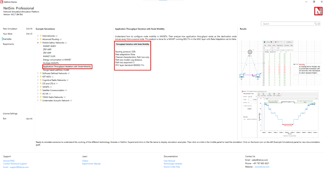
The following network diagram illustrates what the NetSim UI displays when you open the example configuration file see Figure 4-25.

Network Settings
The device coordinates were set as follows. To configure the below, click on device, expand the property panel on right and change the below in position layer.
| Device | X-Coordinate | Y-Coordinate |
|---|---|---|
| N1 | 10 | 150 |
| N2 | 30 | 150 |
Set grid length to 300m\(\times\)150m from grid setting property panel on the right. This needs to be done before any device is placed on the grid.
To configure any properties in the nodes, click on the node, expand the property panel on the right side, and change the properties as mentioned below.
IEEE standard was set to 802.11n in Interface (Wireless) \(\triangleright\) Physical layer of both the wireless nodes.
The Physical layer properties were set as shown in Table 4-2.
| Interface Parameters | Value |
|---|---|
| Standard | IEEE802.11n |
| No. of Frames to Aggregate | 1 |
| Transmitter Power | 100mW |
| Bandwidth | 20MHz |
| Standard Channel | 1 (2412MHz) |
| Reference distance (d0) | 1m |
| Guard Interval | 400ns |
| Antenna | |
| Antenna height | 1m |
| Antenna gain | 0 |
| Transmitting antennas | 1 |
| Receiving antennas | 1 |
The Medium Access Protocol was set to DCF in Interface (Wireless)\(\rightarrow\) Datalink layer of both wireless nodes.
Click on N1 and expand right-hand side property panel and go to Network layer, Enable Static IP Route and Configure Static Route via GUI as shown below screenshot Figure 4-26.

Rate Adaptation was set as False in Interface (Wireless) \(\rightarrow\) Datalink layer of both wireless nodes.
Click on link and expand right-hand side property panel and set the Channel characteristics as: Path loss only; Path loss model: Log Distance; Path loss exponent: 3 under medium property.
Click on the N1 and N2 devices and expand right-hand side property panel and set the mobility model to No Mobility in N1 and File Based Mobility in N2.
Click on set traffic tab and configure Unicast CBR application from N1 to N2. Click on the created application, and in the right-side property panel, set the transport protocol to UDP and the start time to 0s. Set the packet size to 1460 bytes and Inter Arrival Time to 476.2 microseconds, which gives a Generation Rate of 25Mbps.
Set application start time as 0 sec.
The Transport protocol was set to UDP.
Enable the Application throughput vs time plot and SNR vs time plot under Plots in Configure reports.
Run the simulation for 45 seconds.
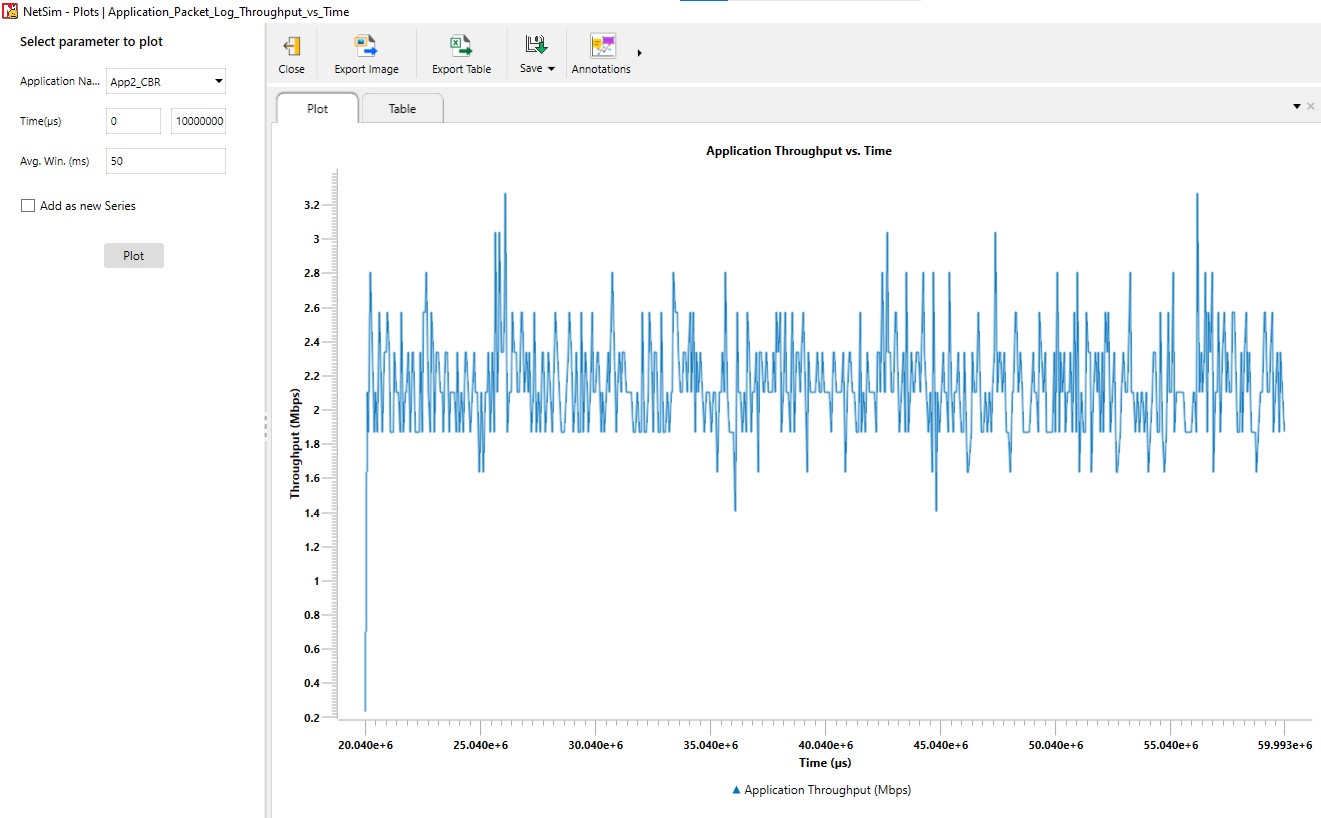
Open the Application throughput vs. Time plot and uncheck the Accelerate plotting and observe the below plot.
File based mobility file
| Time(s) | Node ID | X (m) | Y (m) | Z (m) |
|---|---|---|---|---|
| 0 | 2 | 30 | 100 | 0 |
| 2 | 2 | 40 | 100 | 0 |
| 4 | 2 | 50 | 100 | 0 |
| 6 | 2 | 60 | 100 | 0 |
| 8 | 2 | 70 | 100 | 0 |
| 10 | 2 | 80 | 100 | 0 |
| 12 | 2 | 90 | 100 | 0 |
| 14 | 2 | 100 | 100 | 0 |
| 16 | 2 | 110 | 100 | 0 |
| 18 | 2 | 120 | 100 | 0 |
| 20 | 2 | 130 | 100 | 0 |
| 22 | 2 | 120 | 100 | 0 |
| 24 | 2 | 110 | 100 | 0 |
| 26 | 2 | 100 | 100 | 0 |
| 28 | 2 | 90 | 100 | 0 |
| 30 | 2 | 80 | 100 | 0 |
| 32 | 2 | 70 | 100 | 0 |
| 34 | 2 | 60 | 100 | 0 |
| 36 | 2 | 50 | 100 | 0 |
| 38 | 2 | 40 | 100 | 0 |
| 40 | 2 | 30 | 100 | 0 |
Output


Inference
We can also observe the SNR vs. Time plot obtained after the simulation. The SNR is high initially and gradually drops as N2 moves away from N1. After N2 moves back towards the transmitter around the 20th second, we observe an increase in the SNR. The pathloss exponent in the log distance pathloss model was set to 3.0.
Recall that throughput is proportional to SNR. We observe that the Application throughput drops from 25 Mbps to 20 Mbps at around 4 seconds (the distance at this time is 50 m), and then to 15.8 Mbps at 6.5 seconds (the distance at this time is 70 m) and to 10.2 Mbps at 12 seconds (the distance at this time is 90 m) and then to 5.8 Mbps at 20 seconds (the distance at this time is 130 m). After the 20th second N2 starts moving back towards N1 and we can see the increase in throughput.
Performance of range based pathloss model in MANETs
Open NetSim and Select Examples\(\rightarrow\)Mobile Ad hoc Networks\(\rightarrow\)Range Based pathloss model then click on the tile in the middle panel to load the example as shown in below screenshot Figure 4-28.

Introduction
The propagation loss depends only on the distance (range) between transmitter and receiver. There is a single Range attribute that determines the path loss.
This is not a real-world loss model but a theoretical model useful for experimentation. Receivers at or within Range meters see a 0 dB pathloss. Hence received power equals transmit power. Receivers beyond Range see a 1000 dB pathloss. Hence received power will be close to \(-1000\) dBm i.e., zero in linear units.

The Range-Based Path Loss Model can be used in networks such as Internetworks, MANET, VANET, TDMA, Pure ALOHA, Slotted ALOHA, Cognitive Radio, IoT, WSN, and UWAN.
In this example, we will study the different cases in Range based Pathloss using Mobile Ad hoc networks.
Case 1: Range Based Pathloss. Nodes Within Transmission Range.
The following network diagram illustrates what the NetSim UI displays when you open the example configuration file.

Network Settings
Set grid length as 400 \(\times\) 200 from grid setting property panel on the right. This needs to be done before any device is placed on the grid.
Drop 2 wireless nodes and 1 Ad hoc link in Grid environment.
Device placements of wireless nodes are:
| Device | X-Coordinate | Y-Coordinate |
|---|---|---|
| Wireless Node-1 | 100 | 150 |
| Wireless Node-2 | 180 | 150 |
Click on link and expand right-hand side property panel and set Channel Characteristics: Pathloss, Pathloss model to Range based, Range(m)=100 under medium property.
Clicking on Wireless node and expand right-hand side property panel and set, Mobility Model: No-Mobility, for both nodes under position property.
Click on the set traffic tab present in the top ribbon. Create a CBR Application with 11Mbps generation rate (Set Packet size: 1460, Inter Arrival Time: 1061.81 \(\mu\)s) from wireless node-1 to wireless node-2. Set Transport protocol to UDP and start time to zero.
Enable throughput vs time plot under Application and link performance by clicking on plots/logs tab in right panel.
Run the simulation for 100 seconds.
Output and Plot

In Simulation result window, click on Throughput vs Time plot under Application performance. After the plot window is displayed, click on the plot option.

Discussion
The above results show continuous data transmission and constant throughput throughout the simulation. This occurs because Wireless Node-2 is within the transmission range of Wireless Node-1. Specifically, the range-based parameter is set to 100 meters, and Wireless Node-2 is positioned 80 meters away from Wireless Node-1.
Case 2: Range Based Pathloss. Nodes Beyond Transmission Range.
The following network diagram illustrates what the NetSim UI displays when you open the example configuration file.
Network Settings
Set Grid length as 400 \(\times\) 200 from grid setting property panel on the right. This needs to be done before any device is placed on the grid.
Drop 2 wireless nodes and 1 Ad hoc link in Grid environment.
Device placements of wireless nodes are:
| Device | X-Coordinate | Y-Coordinate |
|---|---|---|
| Wireless Node-1 | 100 | 150 |
| Wireless Node-2 | 180 | 150 |
Click on link and expand right-hand side property panel and set channel characteristics: Pathloss, Pathloss model to Range based, Range(m)=50 meters under medium property.
Click on wireless node and expand right-hand side property panel and set Mobility model: No-mobility, for both nodes under position property.
Click on the set traffic tab present in the top ribbon, create a CBR Application with 11Mbps generation rate (Set Packet size: 1460, Inter Arrival Time: 1061.81 \(\mu\)s) from wireless node-1 to Wireless node-2. Set Transport protocol to UDP and start time to zero.
In NetSim GUI Application and link throughput vs time plot should be enabled.
Run the Simulation for 100 seconds.
Output and Plot

Discussion
From the results, it is evident that there is no data transmission since wireless node-2 is outside the range of wireless node-1. The range-based parameter is set to 50 meters, whereas wireless node-2 is placed 80 meters away from wireless node-1.
Case 3: Range Based Pathloss with Node Mobility.
The following network diagram illustrates what the NetSim UI displays when you open the example configuration file.
Network Settings
Set grid length as 400 \(\times\) 200 from grid setting property panel on the right. This needs to be done before any device is placed on the grid.
Drop 2 wireless nodes and 1 Ad hoc link in Grid environment.
Device placements of wireless nodes are:
| Device | X-Coordinate | Y-Coordinate |
|---|---|---|
| Wireless Node-1 | 100 | 150 |
| Wireless Node-2 | 180 | 150 |
Click on link and expand right-hand side property panel and set Channel Characteristics: Pathloss, Pathloss model to Range based, Range(m)=100 under medium property.
Click on Wireless node and expand right-hand side property panel and set Mobility model: No-mobility to Wireless node 1 and Mobility model: File based mobility to wireless node 2 under position property.
The file-based mobility pattern specifies that at the 0th second, wireless node 2 will be within range, and at the 5th second, it will move out of range. This cycle of moving in and out of range every 5 seconds repeats continuously for 50-seconds.

Click on the set traffic tab present in the top ribbon, create a CBR Application with 11Mbps generation rate (Set packet size: 1460, Inter Arrival Time: 1061.81 \(\mu\)s) from wireless node-1 to wireless node-2. Set Transport protocol to UDP and set start time to zero.
Clicking on wireless node 1 will open a right-hand side property panel and go to Network layer, enable Static IP Route and configure static route via GUI from Wireless node 1 to Wireless node 2 as shown in below table.
| Devices | Network Dest. | Gateway | Subnet Mask | Metrics | Intf. ID |
|---|---|---|---|---|---|
| Wireless node 1 | 192.169.0.3 | 192.169.0.3 | 255.255.255.255 | 1 | 1 |
In NetSim GUI Application and link throughput vs time plot should be enabled.
Run the Simulation for 55 seconds.
Output and Plot


Discussion
The observed results from the plot indicate that data transmission commences at the 0th second and continues until the 5th second, followed by a pause in transmission until the 10th second. Transmission then resumes from the 15th second and ends at the 20th second. This pattern repeats until the 50th second. This behavior aligns with the mobility pattern defined for wireless node-2, in which it is within a 100-meter range of wireless node-1 for the first 5 seconds, and then moves out of range for the next 5 seconds, and so forth.
Case 4: Range Based Pathloss with Multi-hop Communication.
The following network diagram illustrates what the NetSim UI displays when you open the example configuration file.

Network Settings
Set grid length as 400 \(\times\) 200 from grid setting property panel on the right. This needs to be done before any device is placed on the grid.
Drop 3 wireless nodes and 1 Ad hoc link in grid environment.
Device placements of wireless nodes are:
| Device | X-Coordinate | Y-Coordinate |
|---|---|---|
| Wireless Node-1 | 100 | 150 |
| Wireless Node-2 | 140 | 150 |
| Wireless Node-3 | 180 | 150 |
Click on link and expand right-hand side property panel and set Channel characteristics: pathloss, pathloss model to Range based, Range(m)=50 under medium property.
Click on wireless node and expand right-hand side property panel and set Mobility model: No-mobility to 3 devices under position property.
Configure an application between any two nodes by selecting a CBR application with 11Mbps generation rate (Set packet size: 1460, Inter arrival time: 1061.81 \(\mu\)s) from wireless node-1 to wireless node-3 from the set traffic tab. Set transport protocol to UDP and set start time to zero.
Clicking on wireless node 1 and wireless node 2 will open a right-hand side property panel and go to Network layer, enable Static IP Route and configure static route via GUI from wireless node 1 to wireless node 2 and from wireless node 2 to wireless node 3 as shown in below table.
| Devices | Network Dest. | Gateway | Subnet Mask | Metrics | Intf. ID |
|---|---|---|---|---|---|
| Wireless node 1 | 192.169.0.4 | 192.169.0.3 | 255.255.255.255 | 1 | 1 |
| Wireless node 2 | 192.169.0.4 | 192.169.0.4 | 255.255.255.255 | 1 | 1 |
Enable throughput vs time plot under Application and link performance by clicking on plots/logs tab in right panel.
Run the simulation for 100 seconds.
Output and Plot


In the packet trace, filter packets of type Control Packet Type/APP Name to APP1 CBR. Now you can observe multi-hop communication between node 1 and wireless node 3 via node 2. The configuration involves an application from wireless node 1 to wireless node 3, with a range-based parameter set at 50 meters. The direct distance between wireless node 1 and wireless Node 3 is 80 meters, which exceeds the specified range. However, wireless node 2 is within range of both wireless node 1 and wireless node 3, acting as an intermediate node. Therefore, wireless node 1 utilizes wireless node 2 for data transmission, enabling effective multi-hop communication despite the distance constraints.


Case 5: Range Based Pathloss with Multi-hop Communication and Node Mobility
The following network diagram illustrates what the NetSim UI displays when you open the example configuration file.

Network Settings
Set grid length as 500 \(\times\) 250 from grid setting property panel on the right. This needs to be done before any device is placed on the grid.
Drop 3 wireless nodes and 1 Ad hoc link in Grid environment.
Device placements of wireless nodes are:
| Device | X-Coordinate | Y-Coordinate |
|---|---|---|
| Wireless Node-1 | 0 | 200 |
| Wireless Node-2 | 50 | 200 |
| Wireless Node-3 | 100 | 200 |
Click on link and expand right-hand side property panel and set Channel characteristics: Pathloss, Pathloss model to Range based, Range(m)=50 under medium property.
Click on wireless node and expand right-hand side property panel and set mobility model: No-mobility for wireless node 1 and mobility model: File based mobility for wireless node 2 and wireless node 3 under position property.
The file-based mobility file specifies the following sequence: At the 0th second, both wireless node 2 (WN2) and wireless Node 3 (WN3) will be out of range. By the 10th second, wireless node 2 will move within range of wireless node 1, while wireless node 3 remains out of range. Starting from the 20th second, wireless node 2 will stay within range, and wireless node 3 will also come into range of wireless node 2. This setup dictates the mobility and connectivity pattern for the nodes throughout the simulation.

Click on the set traffic tab present in the top ribbon, create CBR application with 11Mbps generation rate (set packet size: 1460, Inter arrival time: 1061.81 \(\mu\)s) from wireless node-1 to wireless node-2 and wireless node-1 to wireless node-3. Set Transport protocol to UDP and set start time to zero.
Clicking on wireless node 1 and wireless node 2 will open a right-hand side property panel and go to Network layer, enable static IP route and configure static route via GUI from wireless node 1 to wireless node 2 and from wireless node 2 to wireless node 3 as shown in below table.
| Devices | Network Dest. | Gateway | Subnet Mask | Metrics | Intf. ID |
|---|---|---|---|---|---|
| Wireless node 1 | 192.169.0.4 | 192.169.0.3 | 255.255.255.255 | 1 | 1 |
| Wireless node 1 | 192.169.0.3 | 192.169.0.3 | 255.255.255.255 | 1 | 1 |
| Wireless node 2 | 192.169.0.4 | 192.169.0.4 | 255.255.255.255 | 1 | 1 |
In NetSim GUI Application throughput vs time and Link throughput vs time plots should be enabled.
Run the simulation for 60 seconds.
Output and Plot


Case 6: Range Based Pathloss. Nodes within range and beyond range. Broadcast Application
The following network diagram illustrates what the NetSim UI displays when you open the example configuration file.

Network Settings
Set grid length as 600 \(\times\) 300 from grid setting property panel on the right. This needs to be done before any device is placed on the grid.
Drop 3 wireless nodes and 1 ad hoc link in grid environment.
Device placements of wireless nodes are:
| Device | X-Coordinate | Y-Coordinate |
|---|---|---|
| Wireless Node-1 | 0 | 200 |
| Wireless Node-2 | 50 | 200 |
| Wireless Node-3 | 200 | 200 |
Click on link and expand right-hand side property panel and set Channel characteristics: Pathloss, Pathloss model to Range based, range(m)=100 under medium property.
Click on wireless node and expand right-hand side property panel and set Mobility model: No-mobility for all the nodes under position property and set Interface-1(wireless), Data link layer, Medium access protocol to DCF.
Click on the set traffic tab present in the top ribbon, create broadcast CBR application with 11Mbps generation rate (Set packet size: 1460, Inter arrival time: 1061.81 \(\mu\)s) from wireless node-2. Set Transport protocol to UDP and set start time to zero.
Run the simulation for 100 seconds.
Output

From the packet trace analysis, it is evident that data transmission occurs between wireless node 1 (WN1) and wireless node 2 (WN2), but not between WN2 and WN3. This outcome is due to the broadcast application configured from WN2, with a range-based path loss setting of 100 meters. Since WN1 is within this range of WN2, data transmission is successfully occurring. However, WN3 is positioned outside the 100-meter range, resulting in no data transmission between WN2 and WN3.
Case 7: Range Based Pathloss. Transmission Failure due to Interference.
The following network diagram illustrates what the NetSim UI displays when you open the example configuration file.

Network Settings
Set grid length as 400 \(\times\) 200 from grid setting property panel on the right. This needs to be done before any device is placed on the grid.
Drop 4 wireless nodes and 1 Ad hoc link in grid environment.
Device placements of wireless nodes are:
| Device | X-Coordinate | Y-Coordinate |
|---|---|---|
| Wireless Node-1 | 0 | 150 |
| Wireless Node-2 | 50 | 150 |
| Wireless Node-3 | 110 | 150 |
| Wireless Node-4 | 140 | 150 |
Click on link and expand right-hand side property panel and set Channel Characteristics: Pathloss, Pathloss model to Range Based, Range(m)=100.
Click on Wireless node and expand right-hand side property panel and set Mobility Model: No-Mobility for all the nodes under position property and set Interface-(Wireless), Data Link Layer, Medium access protocol to DCF.
Click on the set traffic tab present in the top ribbon, create CBR application with 11Mbps generation rate (Set Packet size: 1460, Inter Arrival Time: 1061.81 \(\mu\)s) from Wireless Node-1 to Wireless Node-2 and Wireless Node-3 to Wireless Node-4. Set Transport Protocol to UDP and Set start time to zero.
Run the Simulation for 100 seconds.
Output
In this scenario we have traffic from WN1 to WN2 and from WN3 to WN4. Note however that WN2 is within the range of WN3. In this scenario there is no successful data transmission between WN1 to WN 2. This is because WN2 is within the range of WN 3 which is transmitting to WN4. Packets sent from WN1 cannot be successfully received (decoded) at WN2 due to the interference of the WN3 to WN4 transmission.
Case 8: Range Based Pathloss. Carrier sense (CS) blocking due to neighboring transmissions.
The following network diagram illustrates what the NetSim UI displays when you open the example configuration file.

Network Settings
Set grid length as 400 \(\times\) 200 from grid setting property panel on the right. This needs to be done before any device is placed on the grid.
Drop 4 wireless nodes and 1 Ad hoc link in Grid environment.
Device placements of wireless nodes are:
| Device | X-Coordinate | Y-Coordinate |
|---|---|---|
| Wireless Node-1 | 50 | 150 |
| Wireless Node-2 | 0 | 150 |
| Wireless Node-3 | 100 | 150 |
| Wireless Node-4 | 160 | 150 |
Click on link and expand right-hand side property panel and set Channel Characteristics: Pathloss, Pathloss model to Range Based, Range(m)=100.
Click on Wireless node and expand right-hand side property panel and set Mobility Model: No-Mobility for all the nodes under position property and set Interface-(Wireless), Data Link Layer, Medium access protocol to DCF.
Click on the set traffic tab present in the top ribbon, create CBR Application with 11Mbps generation rate (Set Packet size: 1460, Inter Arrival Time: 1061.81 \(\mu\)s) from Wireless Node-1 to Wireless Node-2 and Wireless Node-3 to Wireless Node-4. Set Transport Protocol to UDP and Set start time to zero.
Run the Simulation for 100 seconds.
Output
We observe that Wireless Node 1 (WN1) is within the range of Wireless Node 2 (WN2) and Wireless Node 3 (WN3), and WN3 is also within range of Wireless Node 4 (WN4). We have configured one application from WN1 to WN2 and another from WN3 to WN4.
In this scenario, WN1 is within the carrier sense range of both WN3 and WN4. Consequently, when WN3 transmits data to WN4, WN1 will delay its transmission due to carrier sense blocking, as it detects the active transmission nearby. Similarly, when WN1 is transmitting data to WN2, WN3 will wait before transmitting to WN4, as it is within the carrier sense range of WN1.

On the other hand, with only WN1-WN2 transmission the obtained throughput is \(5.92\) Mbps and with only WN3-WN4 transmission the throughput is \(5.91\) Mbps. We see that when both transmissions are occurring simultaneously the individual throughputs drop to \(3.62\) Mbps and \(3.59\) Mbps due to carrier sense blocking.
OLSRv2 Multi-cluster MANET
Scenario Overview
The OLSRv2 Multi-cluster MANET example is a 15-node pure wireless MANET simulation that demonstrates the key features of the Optimized Link State Routing Protocol Version 2 (OLSRv2), as implemented in NetSim Pro v15.0.
The network is arranged as three clusters connected by dedicated relay nodes. There is no wired infrastructure; every node is a wireless ad-hoc peer. The scenario uses a deterministic three-phase design: the topology is stable during each phase, with a single, precisely controlled node movement triggering each phase transition. This eliminates randomness and makes every protocol event predictable and verifiable.
Propagation Model – Range-Based Pathloss
The scenario uses range-based pathloss with a fixed range of \(250\) m. This is a deterministic, binary propagation model:
Two nodes within \(250\) m of each other can communicate (link exists, perfect quality).
Two nodes farther than \(250\) m apart cannot communicate (no link).
Configured via the wireless link’s
<MEDIUM PROPERTY> element:
PATHLOSS MODEL="RANGE BASED" RANGE="250"The range applies globally to all nodes on the same wireless link. Combined with file-based mobility, the topology at every instant is fully determined by the node coordinates.
Mobility Model – File-Based
Instead of random mobility, this scenario uses file-based mobility
(FILE BASED MOBILITY). A CSV file specifies the exact
position of each moving node at exact times. Positions change
instantaneously at the specified time with no interpolation and no
randomness. Only Node 5 moves. All other 14 nodes are static. The
mobility file contains three entries that define the three phases.
What This Example Demonstrates
Flooding MPR and Routing MPR selection under varying willingness values.
The catastrophic effect of
WILL_NEVERwhen the willing bridge fails.The effect of TC hop limit truncation.
Triggered TC messages and route recomputation after a deterministic topology change.
Energy consumption differences across node roles.
The full NHDP neighbour discovery lifecycle.
Clean before, during, and after metrics for each phase.
Simulation Configuration
Use the following simulation configuration for the OLSRv2 Multi-cluster MANET example:
15 wireless nodes in a MANET scenario with OLSRv2 as the routing protocol.
Wireless link properties:
Standard: 802.11g
Pathloss model: Range Based
Range: 250 m
Channel characteristics: Pathloss only
Propagation medium: Air
All 15 nodes placed at the Phase 1 coordinates shown below.
Willingness per node:
Nodes 7 and 13:
WILL_FLOODING = WILL_ROUTING = 15Node 6:
WILL_FLOODING = WILL_ROUTING = 0All others: default value 7
TC HOP LIMIT = 4on Node 5 only.Mobility file:
ConfigSupport\mobility.csv.Node 5 mobility:
FILE BASED MOBILITY. All other nodes:NO MOBILITY.Four CBR/UDP flows with start time \(t=20\) s.
Link quality disabled.
Simulation time: 300 s.
Network Topology – Phase 1 (Baseline)
Parameter Configuration
| Parameter | Value | Rationale |
|---|---|---|
| Hello Interval | 2 s | Default |
| Hello Min Interval | 0.5 s | Default (HELLO INTERVAL / 4) |
| HP Maxjitter | 0.5 s | Default (HELLO INTERVAL / 4) |
| TC Interval | 5 s | Default |
| TC Min Interval | 1.25 s | Default (TC INTERVAL / 4) |
| TP Maxjitter | 0.5 s | Same as HP Maxjitter |
| TC Hop Limit | 255 (Node 5: 4) | Demonstrates hop-limit truncation |
| T hold time | 15 s | Default (3 \(\times\) TC INTERVAL) |
| A hold time | 15 s | Default |
| Link Quality | Disabled | Default; not useful with range-based pathloss |
| Pathloss Model | Range-Based | Deterministic binary model |
| Range | 250 m | Produces the designed topology |
| Wireless Standard | 802.11g | Typical MANET radio |
| Mobility (Node 5) | File-Based | See the mobility listing below |
| Mobility (all others) | No Mobility | Static nodes |
| Simulation Time | 300 s | Three phases with ample measurement windows |
Topology Diagram

WILL_NEVER prevents relaying.Node Placement
| Node | X | Y | Role | Willingness |
|---|---|---|---|---|
| 1 | 300 | 1280 | Cluster A hub | DEFAULT (7) |
| 2 | 150 | 1100 | Cluster A core | DEFAULT (7) |
| 3 | 450 | 1100 | Cluster A core | DEFAULT (7) |
| 4 | 100 | 930 | Cluster A edge | DEFAULT (7) |
| 5 | 300 | 950 | Cluster A / bridge to B | DEFAULT (7) |
| 6 | 480 | 870 | Cluster A / alt. bridge | NEVER (0) |
| 7 | 300 | 730 | Relay A–B | ALWAYS (15) |
| 8 | 150 | 560 | Cluster B core | DEFAULT (7) |
| 9 | 450 | 560 | Cluster B core | DEFAULT (7) |
| 10 | 80 | 390 | Cluster B edge | DEFAULT (7) |
| 11 | 300 | 390 | Cluster B edge | DEFAULT (7) |
| 12 | 520 | 390 | Cluster B / bridge to C | DEFAULT (7) |
| 13 | 650 | 220 | Relay B–C | ALWAYS (15) |
| 14 | 530 | 50 | Cluster C | DEFAULT (7) |
| 15 | 770 | 50 | Cluster C | DEFAULT (7) |
| Region | Link | Distance (m) | Note |
|---|---|---|---|
| Cluster A | 1–2 | 234 | |
| Cluster A | 1–3 | 234 | |
| Cluster A | 2–4 | 177 | |
| Cluster A | 2–5 | 212 | |
| Cluster A | 3–5 | 212 | |
| Cluster A | 3–6 | 232 | |
| Cluster A | 4–5 | 201 | |
| Cluster A | 5–6 | 197 | |
| Bridge A–B | 5–7 | 220 | Primary bridge |
| Bridge A–B | 6–7 | 228 | WILL_NEVER; cannot relay |
| Cluster B | 7–8 | 227 | |
| Cluster B | 7–9 | 227 | |
| Cluster B | 8–10 | 184 | |
| Cluster B | 8–11 | 227 | |
| Cluster B | 9–11 | 227 | |
| Cluster B | 9–12 | 184 | |
| Cluster B | 10–11 | 220 | |
| Cluster B | 11–12 | 220 | |
| Bridge B–C | 12–13 | 214 | Sole bridge |
| Cluster C | 13–14 | 208 | |
| Cluster C | 13–15 | 208 | |
| Cluster C | 14–15 | 240 |
Adjacency List
| Pair | Distance (m) | Why It Matters |
|---|---|---|
| 2–3 | 300 | Forces Node 1 to need both 2 and 3 as MPRs |
| 1–5 | 330 | Node 1 cannot reach the bridge directly |
| 4–7 | 283 | No shortcut from Cluster A edge to relay |
| 6–8 | 453 | WILL_NEVER node isolated from
Cluster B |
| 8–9 | 300 | Cluster B cores are not directly connected |
| 7–11 | 340 | Relay cannot skip the Cluster B core |
| 9–13 | 394 | No shortcut from Cluster B to relay C |
Simulation Phases
The simulation is divided into three phases, each with a stable topology. Transitions between phases are triggered by a single, instantaneous position change of Node 5.
| Phase | Time Window | Node 5 Position | Topology State |
|---|---|---|---|
| 1 – Baseline | \(t=0\) to \(t=50\) s | \((300,950)\) | Full connectivity (22 links) |
| 2 – Bridge Break | \(t=50\) to \(t=150\) s | \((300,1000)\) | A–B disconnected (21 links) |
| 3 – Recovery | \(t=150\) to \(t=300\) s | \((300,950)\) | Full connectivity restored (22 links) |
Mobility File
The entire mobility specification is a three-line CSV file. Only Node
5 has entries; all other nodes use NO MOBILITY.
#Time(s),Device ID,X,Y,Z
0,5,300,950,0
50,5,300,1000,0
150,5,300,950,0
Node 5 is configured with:
<MOBILITY MODEL="FILE BASED MOBILITY" OPEN MOBILITY FILE="ConfigSupport\mobility.csv" />Phase 1 – Baseline (\(t=0\) to \(50\,s\))
Topology: the full 22-link network. Node 5 at \((300,950)\) is within 220 m of Node 7, so the primary A–B bridge is active.
Protocol activity:
\(t=0\) to \(16\) s: NHDP convergence. HELLO messages propagate hop by hop and links transition
PENDING\(\rightarrow\)HEARD\(\rightarrow\)SYMMETRIC. WithHELLO INTERVAL = 2 sand a 7-hop diameter, full symmetric neighbour discovery completes by approximately 16 s.\(t=5\) to \(20\) s: TC propagation. The first TC messages are generated at approximately 5 s. They flood via MPRs across the 7-hop chain, and routing tables populate progressively.
\(t=20\) s: all application flows start. The network is in steady state.
\(t=20\) to \(50\) s: baseline measurement window (30 s).
Steady-state routing paths:
| Flow | Path | Hops | Status |
|---|---|---|---|
| F1 (10\(\rightarrow\)15) | 10\(\rightarrow\)11\(\rightarrow\)12\(\rightarrow\)13\(\rightarrow\)15 | 4 | Active |
| F2 (4\(\rightarrow\)11) | 4\(\rightarrow\)5\(\rightarrow\)7\(\rightarrow\)8\(\rightarrow\)11 (or via 9) | 4 | Active |
| F3 (14\(\rightarrow\)1) | 14\(\rightarrow\)13\(\rightarrow\)12\(\rightarrow\)9\(\rightarrow\)7\(\rightarrow\)5\(\rightarrow\)2\(\rightarrow\)1 | 7 | Active |
| F4 (3\(\rightarrow\)8) | 3\(\rightarrow\)5\(\rightarrow\)7\(\rightarrow\)8 | 3 | Active |
Phase 2 – Bridge Break (\(t=50\) to \(150\,s\))
At \(t=50\) s, Node 5 moves instantaneously from \((300,950)\) to \((300,1000)\), a shift of 50 m north.
| Link | Before (m) | After (m) | Status | Comment |
|---|---|---|---|---|
| 5–7 | 220 | 270 | BROKEN | Exceeds 250 m |
| 5–2 | 212 | 180 | OK | Closer |
| 5–3 | 212 | 180 | OK | Closer |
| 5–4 | 201 | 212 | OK | Slightly farther |
| 5–6 | 197 | 222 | OK | Slightly farther |
| 1–5 | 330 | 280 | Still out | Still greater than 250 m |
The WILL_NEVER Trap
After the bridge break, the only physical link between Cluster A and
Node 7 is 6\(\leftrightarrow\)7 (228 m,
still within range). But Node 6 has WILL_NEVER = 0:
Node 6 is not an MPR, so it does not relay TC messages.
Node 6 does not forward data packets.
The link 6–7 is physically present but useless for transit.
As a result, Clusters A and B+C become disconnected for all transit
traffic. This is the most dramatic demonstration of
WILL_NEVER: a single willing bridge fails, and the
physically available alternative cannot compensate.
Protocol Events at \(t=50\) s
Node 5 and Node 7 detect link loss via NHDP (HELLO timeout, approximately 6 s =
H HOLD TIME).Link status transitions
SYMMETRIC\(\rightarrow\)HEARD\(\rightarrow\)LOST.Node 7 increments its ANSN (Advertised Neighbour Sequence Number) and generates a triggered TC message.
Node 5 also generates a triggered TC because it lost Node 7 as a neighbour.
The triggered TCs propagate via MPRs: Node 7’s TC reaches Clusters B and C, while Node 5’s TC reaches Cluster A. Neither TC crosses the broken bridge.
Every node that receives the TC recomputes its routing table using Dijkstra.
Routes between Clusters A and B/C are removed because no valid next hop exists.
| Time | Event |
|---|---|
| \(t=50\) s | Node 5 moves; link 5–7 physically breaks |
| \(t\approx52\) s | Next HELLO from Node 5 is not heard by Node 7, and vice versa |
| \(t\approx56\) s | L_SYM time expires on both ends, moving to
HEARD |
| \(t\approx56\) s | H HOLD TIME (6 s) expires,
moving to LOST |
| \(t\approx56\) s | Triggered TC messages from Nodes 5 and 7 |
| \(t\approx58\) to \(65\) s | TC propagation and route settling complete across the remaining topology |
| \(t\approx58\) to \(65\) s | Routing tables update and flows F2, F3, and F4 begin dropping packets after reconvergence |
| Flow | Status | Reason |
|---|---|---|
| F1 (10\(\rightarrow\)15) | Active | Path 10\(\rightarrow\)11\(\rightarrow\)12\(\rightarrow\)13\(\rightarrow\)15 remains within B+C |
| F2 (4\(\rightarrow\)11) | BROKEN | Requires the A\(\rightarrow\)B bridge; no willing path exists |
| F3 (14\(\rightarrow\)1) | BROKEN | Requires the B\(\rightarrow\)A bridge; no willing path exists |
| F4 (3\(\rightarrow\)8) | BROKEN | Requires A\(\rightarrow\)B bridging; Node 6 cannot relay |
Phase 3 – Recovery (\(t=150\) to \(300\,s\))
At \(t=150\) s, Node 5 returns instantaneously to \((300,950)\) and link 5–7 reforms.

WILL_NEVER blocks all relaying.Protocol Events at \(t=150\) s
Node 5’s HELLO reaches Node 7 again. The link transitions
LOST\(\rightarrow\)HEARD\(\rightarrow\)SYMMETRIC, requiring two HELLO exchanges and approximately 4 s.Both nodes generate triggered TC messages announcing the restored neighbour.
Triggered TCs propagate via MPRs across both sides of the network.
Routing tables are recomputed with the restored bridge, and routes between Clusters A and B/C reappear after the protocol settles.
All four flows recover.
| Time | Event |
|---|---|
| \(t=150\) s | Node 5 moves back; link 5–7 becomes physically available |
| \(t\approx152\) s | Node 5’s HELLO is heard by Node 7, moving
to HEARD |
| \(t\approx154\) s | Symmetric confirmation through the second
HELLO, moving to SYMMETRIC |
| \(t\approx154\) s | Triggered TC messages from Nodes 5 and 7 |
| \(t\approx156\) to \(165\) s | TC propagation and route settling continue |
| \(t\approx156\) to \(165\) s | Routing tables restore and flows F2, F3, and F4 resume delivery |
Measurement window: \(t=165\) to \(300\) s (135 s of restored steady state).
Expected outcome: Phase 3 metrics should closely match Phase 1 metrics for all four flows, confirming that the protocol fully recovers from the disruption.
Features Exercised
MPR Selection – Flooding and Routing
Node 1’s MPR Selection (all phases). Node 1’s one-hop neighbours are {2, 3}. The two-hop set is:
via Node 2: {4, 5}
via Node 3: {5, 6}
The unique two-hop set is {4, 5, 6}. Node 2 covers {4, 5}, and Node 3 covers {5, 6}. Neither alone covers all three, so both are selected as MPRs.
Node 5’s MPR Selection (Phases 1 and 3). The one-hop
neighbours are {2, 3, 4, 6, 7}. The two-hop set is {1, 8, 9}. Node 2 or
Node 3 covers {1}, while Node 7 covers {8, 9} and has
WILL_ALWAYS, guaranteeing selection. Node 6 provides no
unique two-hop coverage and has WILL_NEVER, so it is never
selected.
Node 5’s MPR Selection (Phase 2). Node 5 loses Node 7 as a neighbour. The new one-hop set is {2, 3, 4, 6}. The new two-hop set is {1, 7}, with Node 7 learned as a two-hop neighbour via Node 6. The MPR set shrinks relative to Phase 1.
Flooding vs. Routing MPRs. OLSRv2 maintains separate
flooding and routing MPR sets (RFC 7181 Sections 18.1 and 18.4). Both
are independently configurable via WILL_FLOODING and
WILL_ROUTING.
Willingness Variation and the WILL_NEVER Trap
WILL_ALWAYS (15) is configured on Nodes 7 and 13,
guaranteeing MPR selection. WILL_NEVER (0) is configured on
Node 6, so it never relays. In Phase 1 this is merely observable; in
Phase 2 it becomes critical because the only physical A–B link is 6–7,
but WILL_NEVER renders it useless for transit,
disconnecting the clusters. All other nodes use
WILL_DEFAULT (7).
TC Hop Limit Truncation
Observe the effect of TC HOP LIMIT for Node 5 by
comparing these two cases:
TC HOP LIMIT = 255: Node 5’s TC propagates normally through the connected topology.TC HOP LIMIT = 4: Node 5’s TC is forwarded only up to the fourth hop. The node at hop 4 may receive the TC, but it does not retransmit it further.
Triggered TC Messages
Periodic TCs are generated every 5 s. However, topology changes
trigger immediate TC messages, subject to
TP MAXJITTER = 0.5 s. This scenario produces two
triggered-TC bursts:
Around \(t\approx56\) to \(65\) s, after the link 5–7 loss.
Around \(t\approx154\) to \(165\) s, after the link 5–7 restoration.
NHDP Neighbour Discovery Lifecycle
Neighbour discovery is observable in three contexts:
Initial convergence (\(t=0\) to \(16\) s): all links transition
PENDING\(\rightarrow\)HEARD\(\rightarrow\)SYMMETRIC.Link loss (around \(t\approx52\) to \(65\) s): link 5–7 transitions
SYMMETRIC\(\rightarrow\)HEARD\(\rightarrow\)LOST.Link recovery (around \(t\approx150\) to \(165\) s): link 5–7 transitions
LOST\(\rightarrow\)HEARD\(\rightarrow\)SYMMETRIC.
Energy Consumption by Role
All nodes use the default NetSim energy model (TX: 316.7 mA, RX: 261.1 mA, Idle: 227 mA, Voltage: 3.6 V).
Phase-dependent expected results:
Node 7 (
WILL_ALWAYSrelay) has the highest TX energy in Phases 1 and 3 because it relays all cross-cluster traffic.In Phase 2, Node 7’s TX energy drops because it no longer relays A\(\rightarrow\)B traffic; only B\(\rightarrow\)C traffic remains.
Node 6 (
WILL_NEVER) has the lowest TX energy in all phases.Node 13 remains consistently active as the B–C bridge, unaffected by Node 5’s movement.
Traffic Flows
Four concurrent CBR/UDP flows start at \(t=20\) s and run for the remainder of the simulation.
| Flow | Src | Dst | Type | Packet Size | Rate | Purpose |
|---|---|---|---|---|---|---|
| F1 | 10 | 15 | CBR/UDP | 512 B | 10 pkt/s | Entirely within B+C (4 hops); unaffected by the bridge break and serves as a control flow |
| F2 | 4 | 11 | CBR/UDP | 512 B | 10 pkt/s | Crosses A\(\rightarrow\)B via Node 7; breaks in Phase 2 |
| F3 | 14 | 1 | CBR/UDP | 512 B | 5 pkt/s | Longest path (7 hops); breaks in Phase 2 |
| F4 | 3 | 8 | CBR/UDP | 256 B | 20 pkt/s | WILL_NEVER bypass
demonstration (3 hops); breaks in Phase 2 |
Per-Phase Flow Behaviour
F1 remains active across all three phases because its path 10\(\rightarrow\)11\(\rightarrow\)12\(\rightarrow\)13\(\rightarrow\)15 never crosses the A–B bridge. F2, F3, and F4 break during Phase 2 and recover in Phase 3 after reconvergence. The windows \(t=50\) to \(65\) s and \(t=150\) to \(165\) s are transient intervals rather than steady-state measurement periods.
Simulation Results – Phase by Phase
Phase 1 Observations (Baseline, \(t=20\) to \(50\,s\))
| Observation | Where to Look | Expected Result |
|---|---|---|
| MPR tables | OLSR link metrics log | Node 1 MPRs = {2, 3}. Node 5 MPRs include
Node 7 (WILL_ALWAYS). Node 6 never appears as an MPR for
any node. |
| WILL_NEVER effect | Routing tables | Node 6 is reachable as a destination but never used as a next hop. Flow F4 uses 3\(\rightarrow\)5\(\rightarrow\)7\(\rightarrow\)8, not 3\(\rightarrow\)6\(\rightarrow\)7\(\rightarrow\)8. |
| TC hop limit | Packet trace | Node 5’s TCs are limited to 4 hops. The node at hop 4 may receive the TC but does not forward it further, so Nodes 14 and 15 are not reached directly. Other nodes’ TCs propagate Node 5’s information farther. |
| Full convergence | Routing table timestamps | All 15 nodes have complete routing tables by approximately \(t=16\) to \(20\) s. |
| All flows active | Application metrics | F1 remains active on its 4-hop path. F2–F4 are also active in the baseline phase on their respective paths. |
| Jitter | Packet trace | HELLO and TC transmission times vary by up to 0.5 s and 0.5 s, respectively, from the periodic schedule. |
Phase 2 Observations (Bridge Break, \(t=50\) to \(150\,s\))
| Observation | Where to Look | Expected Result |
|---|---|---|
| Link 5–7 loss | NHDP logs | SYMMETRIC \(\rightarrow\) HEARD \(\rightarrow\) LOST on both
Node 5 and Node 7 at approximately \(t=56\) s. |
| Triggered TC burst | Packet trace | Non-periodic TCs from Nodes 5 and 7 at approximately \(t=56\) s, clearly distinguishable from the 5 s periodic cadence. |
| ANSN increment | TC message headers | Nodes 5 and 7 increment ANSN in the triggered TCs. |
| MPR table change | OLSR link metrics log | Node 5’s MPR set shrinks because it loses Node 7. Node 7’s MPR set shrinks because it loses Node 5. |
| Route removal | Routing tables | All Cluster A nodes lose routes to Cluster B/C nodes and vice versa. Intra-cluster routes remain intact on both sides. |
| F1 unaffected | Application metrics | F1 remains active throughout because its path is entirely within B+C. |
| F2/F3/F4 broken | Application metrics | Delivery drops after approximately \(t=58\) to \(65\) s once reconvergence completes. |
| Node 7 energy drop | Energy logs | Node 7’s TX energy rate decreases in Phase 2 because it no longer relays A\(\rightarrow\)B data or TCs from Cluster A. |
| WILL_NEVER trap | Routing tables (Node 6) | Node 6 still has a SYMMETRIC
link to Node 7, but its routing table shows no routes to Cluster B/C
because Node 7’s TCs are not relayed back via Node 6. Even if routes
were present, Node 6 would still not forward. |
Phase 3 Observations (Recovery, \(t=150\) to \(300\,s\))
| Observation | Where to Look | Expected Result |
|---|---|---|
| Link 5–7 recovery | NHDP logs | LOST \(\rightarrow\) HEARD \(\rightarrow\) SYMMETRIC on
both ends at approximately \(t=154\)
s. |
| Triggered TC burst | Packet trace | Second burst of non-periodic TCs from Nodes 5 and 7. |
| Route restoration | Routing tables | Cross-cluster routes reappear network-wide after recovery, typically around \(t=156\) to \(165\) s depending on settling time. Paths then match Phase 1 again. |
| F2/F3/F4 resume | Application metrics | Traffic resumes only after reconvergence. The interval around \(t=150\) to \(165\) s shows partial restoration while NHDP re-establishes the link and routing tables settle. |
| Metrics match Phase 1 | All logs | Phase 3 steady-state metrics should closely match Phase 1, confirming full protocol recovery. Persistent differences indicate a convergence defect. |
Running the Example in NetSim
Open the OLSRv2 Multi-cluster MANET example in NetSim Pro v15.0. The example is pre-configured with all node positions, willingness values, mobility, traffic flows, and protocol settings described in this section.
Observing Simulation Results and TC Hop Limit Effects
After running the simulation, the following outputs can be observed:
OLSR link metrics log: displays MPR tables for each phase.
Packet trace: observe the difference between the default hop limit (255) and Node 5 configured with hop limit 4, along with triggered TC bursts at \(t\approx56\) s and \(t\approx154\) s.
Routing table snapshots: tables at different time instances, such as \(t=40\) s, \(t=100\) s, and \(t=200\) s, illustrate routing changes across phases.
Application metrics: show delivery ratio and delay for each flow across phases.
Energy logs: highlight variations in transmission energy across nodes, such as Node 7 versus Node 6.
TC Hop Limit
The TC Hop Limit controls how far a TC (Topology Control) message propagates in the network.
Steps to Verify the Effect
Run the simulation and open the Packet Trace window.
Apply the following filters:
Packet Type =
TC_MESSAGESource Node = 5
Identify the TC messages generated by Node 5.
Track a selected TC packet as it propagates through neighbouring nodes across the network.
Expected Observations
For Node 5 (TC Hop Limit = 4):
The TC message is forwarded only up to four hops from the source node.
When the hop count reaches 4, the packet is received by the node but is not forwarded further.
Nodes located beyond four hops do not receive this TC message directly.
For Other Nodes (Default TC Hop Limit = 255):
TC messages propagate throughout the entire network without early termination.
Verification Method
Compare TC packets generated by Node 5 with TC packets generated by other nodes in the network. Only the TC messages originating from Node 5 will demonstrate early truncation due to the reduced hop limit, confirming the effect of the configured TC Hop Limit.
Conclusion
This example provides a fully deterministic evaluation of OLSRv2. Range-based pathloss and file-based mobility ensure that every topology change is precisely controlled and every protocol event is reproducible.
The three-phase design produces a clean before, during, and after comparison:
Phase 1 establishes the baseline: MPR selection, TC propagation, multi-hop routing, and energy consumption under full connectivity.
Phase 2 shows the protocol’s response to a controlled disruption: triggered TC generation, route removal, ANSN updates, and the catastrophic impact of
WILL_NEVERwhen the sole willing bridge fails.Phase 3 confirms complete recovery: link re-establishment, route restoration, and metric convergence back to baseline.
The control flow F1, which is unaffected by the bridge break, confirms that the disruption is localised to cross-cluster paths.