Featured Examples
Derive from 3GPP standards the theoretical data rate and throughput for a 1gNB - 2UE scenario, and compare with simulation
Introduction
NetSim calculates the PHY rate per the 3GPP formula, which is explained in the infographic below.

A simple, approximate way to think of the above formula is
\[\begin{equation} Data\ Rate = BW \times Q \times R \times N \times (1 - OH) \qquad \ldots (1) \end{equation}\]
where Data rate is the per carrier PHY rate, BW is the allocated bandwidth to the particular UE, Q is the modulation order, R is the code rate, N is the number of MIMO layers, and OH is the Overhead. In NetSim, OH is usually taken as 2/14 since we have 2 control symbols in a slot spanning 14 symbols.
How is the formula in (1) equivalent to the 3GPP formula Let’s examine the variables.
Q, R, N, and (1-OH) are common to both
The scaling factor in NetSim is assumed as 1
The data rate in (1) per carrier and needed to be summed up for multiple carriers
What remains to be shown is that BW is the same as \(N_{prb} \times 12 / T_s\). In this 12 is the number of subcarriers and \(T_s\) represents the symbol duration which varies with numerology. \(10^{-3}\) represents 1 ms, 14 is the number of OFDM symbols and \(2^\mu\) adjusts the slot duration based on the numerology. When we calculate \(N_{prb} \times 12 / T_s\), we are essentially calculating the total number of subcarriers allocated within the given symbol duration, which is nothing, but the bandwidth allocated to that device. The simplified formula we provided would yield a slightly higher estimate compared to the 3GPP formula because of the way \(N_{prb}\) is calculated in the standards.
When operating in TDD mode, the above computation would give the two-way (downlink + uplink) data rate. Therefore, the downlink data rate would be
\[\begin{equation} DL\text{-}rate = Data\ Rate \times DL\text{-}Fraction \qquad \ldots (2) \end{equation}\]
While BW, OH, and N are based on user inputs in NetSim, Q and R are dependent on the modulation and coding scheme (MCS). The MCS i.e., Q and R, is chosen by looking up the 3GPP spectral efficiency to MCS table assuming ideal Shannon rate whereby
\[\begin{equation} Spectral\text{-}Efficiency = \log_2 \left(1 + SINR[linear]\right) \qquad \ldots (3) \end{equation}\]
The expression thus becomes
\[\begin{equation} \frac{DL}{UL} Data\ Rate\ [Mbps] = BW\ [MHz] \times Q\ \left[\frac{bits}{symbol}\right] \times R \times N \times (1 - OH) \times \left(\frac{DL}{UL} fraction\right) \qquad \ldots (4) \end{equation}\]
Bandwidth is the cycles per second which translates to the number of signal changes (or symbol transmissions) per second. Hence multiplying BW and Q gives Mbits/sec when BW is in MHz. The other terms are dimensionless.
Now, in 5G, the transmitter adapts its PHY layer MCS depending on the receiver’s SINR. The SINR in turn depends on the received power, which is transmit-power less pathloss. In NetSim users can record the radio measurements to obtain the SINR and MCS (for each UE) over time if the channel is time varying.
Network Setup
Open NetSim, Select Examples \(\rightarrow\) 5G NR \(\rightarrow\) 5G data rate and throughput computation then click on the tile in the middle panel to load the example as shown in below screenshot.


Network Settings
Grid length is set to 6000m \(\times\) 3000m by clicking on the grid panel on right.
Consider a single Macro cell gNB and two UEs. The distance from the gNB to the first UE should be 1900m, and the distance to the second UE should be 2100m.
Click on the gNB and expand property panel on right and set the properties in 5G RAN layer as mentioned in the below table.
| Properties | ||||||
|---|---|---|---|---|---|---|
| Users | Per user (Mbps) | Agg. (Mbps) | Avg delay (\(\mu\)s) | Per user (Mbps) | Agg. (Mbps) | Avg delay (\(\mu\)s) |
| Datalink Layer Properties | ||||||
| Scheduling type | Round Robin | |||||
| Physical Layer Properties | ||||||
| CA type | Single band | |||||
| CA Configuration | n78 | |||||
| CA1 | ||||||
| Numerology | 1 | |||||
| Channel Bandwidth | 100 MHz | |||||
| Channel Model | ||||||
| Pathloss Model | 3GPP TR 38.901-7.4.1 | |||||
| Outdoor Scenario | Rural macro | |||||
| LOS NLOS Selection | User defined | |||||
| LOS Probability | 1 | |||||
| Shadow Fading Model | 3GPP TR 38.901-7.4.1 | |||||
| Fast Fading Model | No Fading | |||||
Set Transmitter and Receiver antenna count as shown in the below table.
| Device | Tx Antenna Count | Rx Antenna Count |
|---|---|---|
| gNB | 2 | 2 |
| UE 1 | 1 | 1 |
| UE 2 | 2 | 2 |
Create a CBR application for both UEs from the servers by clicking on the Set Traffic tab in the ribbon at the top. Keep the packet size at the default (1460 B) and change the inter-arrival time to 97.33 \(\mu\)s, thereby generating 120 Mbps of data for each UE.
Enable the LTE NR Radio Measurement log by clicking on Configure reports tab and plots.

Run the simulation for 10 seconds.
Results

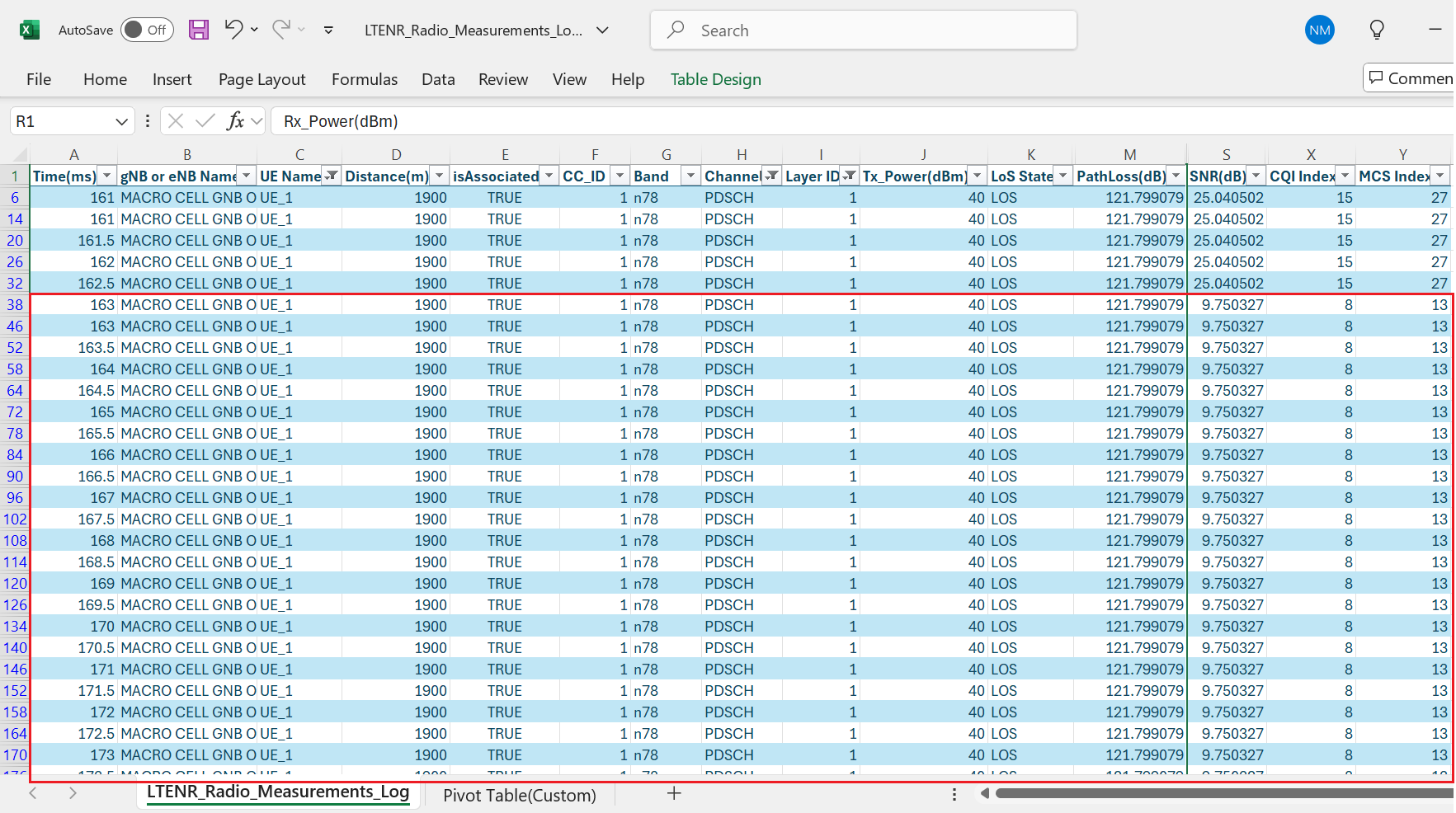
Open LTENR Radio measurement log from simulation results window and filter the channel to PDSCH, Layer ID to 1, To observe the MCS, CQI, Pathloss and SNR values for UE 1, filter the UE ID to UE 1
Filter the UE ID to UE 2, to observe the MCS, CQI, Pathloss and SNR values for UE 2 alone.

NOTE: The values obtained till 163 ms are during RRC association time, hence consider the values after 163 ms.
The PHY Data Rate Calculations for UE 1
\(PHY\ data\ rate(in\ Mbps) = 10^{-6} \sum_{j=1}^{J} (v_{Layers}^{(j)}) \cdot Q_m^{(j)} \cdot f^{(j)} \cdot R \frac{N_{PRB}^{BW(j),\mu} \cdot 12}{T_s^{\mu}} (1 - OH^{(j)})\),
where \(T_s^{\mu} = \frac{10^{-3}}{14 \cdot 2^{\mu}}\)
For UE 1,
The number of layers \(v = 1\), since the Tx and Rx antenna of UE count is \(1 \times 1\), Obtained MCS is 13 which means the \(Q_m\) (Modulation order) is 6, \(f = 1\), \(N_{PRB} = 273\), \(OH\) in downlink for FR1 is 0.14.
\[\begin{equation} Data\ Rate\ [Mbps] = 10^{-6}\left(1 \times 6 \times 1 \times \frac{567}{1024} \times \frac{273 \times 12}{\left(\frac{10^{-3}}{14 \cdot 2^{1}}\right)} \times (1 - 0.14)\right) = 262.08\ \text{Mbps} \end{equation}\]
This is total Data Rate which includes DL and UL. The DL data rate would be
\(DL\ Data\ rate = Data\ Rate\ (Mbps) \times \frac{DL}{DL+UL}\) = \(262.08 \times \frac{4}{5} = 209.66\) Mbps
Since, we have 2 UE, with round robin resource allocation, alternate slots are allocated to each UE, therefore the PHY throughput for UE1 would be
\[\begin{equation} PDSCH\ PHY\ Throughput\ [Mbps] = \frac{DL\ Data\ rate\ [Mbps]}{2} = \frac{209.66}{2} = 104.83\ \text{Mbps} \end{equation}\]
This is PHY layer throughput, and hence Application layer throughput would be
\[\begin{equation} DL\ App\ throughput\ [Mbps] = PDSCH\ PHY\ Throughput \times \frac{App\ layer\ Pkt\ Size}{Phy\ layer\ Pkt\ Size} \end{equation}\]
The PHY Data Rate Calculations for UE 2
For UE 2,
The number of layers \(v = 2\), since the Tx and Rx antenna of UE count is \(2 \times 2\), Obtained MCS is 7 which means the \(Q_m\) (Modulation order) is 4, \(f = 1\), \(N_{PRB} = 273\), \(OH\) in downlink for FR1 is 0.14.
\[\begin{equation} Data\ Rate\ [Mbps] = 10^{-6}\left(2 \times 4 \times 1 \times \frac{490}{1024} \times \frac{273 \times 12}{\left(\frac{10^{-3}}{14 \cdot 2^{1}}\right)} \times (1 - 0.14)\right) = 301.98\ \text{Mbps} \end{equation}\]
This is total Data Rate which includes DL and UL. The DL data rate would be
\(DL\ Data\ rate = Data\ Rate\ (Mbps) \times \frac{DL}{DL+UL}\) = \(301.98 \times \frac{4}{5} = 241.58\) Mbps
Since, we have 2 UE, with round robin resource allocation, alternate slots are allocated to each UE, therefore the PHY throughput for UE1 would be
\[\begin{equation} PDSCH\ PHY\ Throughput\ [Mbps] = \frac{DL\ Data\ rate\ [Mbps]}{2} = \frac{241.58}{2} = 120.79\ \text{Mbps} \end{equation}\]
This is PHY layer throughput, and hence Application layer throughput would be
\[\begin{equation} DL\ App\ throughput\ [Mbps] = PDSCH\ PHY\ Throughput \times \frac{App\ layer\ Pkt\ Size}{Phy\ layer\ Pkt\ Size} \end{equation}\]
Results and discussion
We run a simulation in NetSim per the above scenario and obtain the throughput values tabulated below.
| PHY Data Rate (Analytical throughput) in Mbps | Application throughput (Simulation) in Mbps | |
|---|---|---|
| UE 1 | 101.69 | 95.36 |
| UE 2 | 116.48 | 109.81 |
UE 2 achieves higher throughput despite being further from the gNB due to \(2 \times 2\) MIMO vs \(1 \times 1\) MIMO UE 1.
The application layer throughput would be
\[\begin{equation} DL\ App\ Throughput = DL\ DataRate \times (App\ Layer\ Packet\ Size) \end{equation}\]
\(DL\ App\ throughput = DL\ Data\ Rate \times \frac{App\ layer\ packet\ size}{Phy\ layer\ packet\ size} \qquad \ldots (4)\)
The computation of the PHY layer packet size is complex. It involves various layers adding overheads: the Transport layer (UDP) contributes 8 B, and the Network Layer (IP) adds 20 B. The MAC layer introduces additional overhead, with the SDAP header contributing 1B and the PDCP header adding 16B. At this point, the packet size is the size of the application layer packet plus 45 B. The MAC layer in 5G further processes these packets, fitting them into transport blocks (TBs). These TBs are then divided into code blocks (CBs), which are grouped into code block groups (CBGs) for transmission over the air. The sizes of the TB and CB depend on various parameters, and additional overheads are incurred during this process. As a result, it’s challenging to provide a simple analytical formula for PHY layer packet size. A reasonable estimate would be about 5–10% reduction between the PHY rate and the application throughput. This is what we observe when we compare the simulation results with the theoretical predictions in the above table.
The above discussion assumes a conservative MCS is selected, ensuring a Block Error Rate (BLER) of zero. However, if a more aggressive MCS is chosen, which typically has a higher throughput but also a higher t-BLER (e.g., 5% or 10%), the computation must account for this increased BLER.
Exercises
Explain how changing the DL:UL ratio would affect the results Redo the theoretical calculations for DL:UL ratio of 1:1 and compare against simulation.
Change the gNB UE distances such that the MCSs seen by the UEs are different for e.g., MCS 17 and MCS 23. Compute the theoretical throughput and compare against simulation.
Effect of distance on pathloss, SINR and MCS (7-Cell Hexagonal Layout, Urban Macro Propagation, NLOS)
The experiment aims to analyze how the performance of a UE changes as it moves away from its serving gNB. In real-world scenarios, users are mobile, and their distance from the base station affects signal strength. By simulating a linear movement of the UE away from the gNB, we can observe how parameters such as pathloss, SINR, and MCS change with distance. This helps determine the coverage limit of the gNB, identify when the signal is no longer sufficient for communication, and plan for handover decisions.
Network Layout for UE Coverage Analysis in Multi-Cell Scenario:

The following network diagram illustrates what the NetSim UI displays when you open the example configuration file.

Settings done in example config file
Set distance between all gNB as 1500m
Set the gNB properties as follows. To configure it, click on gNB. On the right side, expand the property panel, go to the physical layer of the Interface (RAN) layer, and set the properties below
| Properties | |
|---|---|
| CA Configuration | n78 |
| Antenna | |
| TX Antenna Count | 1 |
| RX Antenna Count | 1 |
| Channel Model | |
| Pathloss Model | 3GPP TR 38.901-7.4.1 |
| Outdoor Scenario | Urban macro |
| LOS NLOS Selection | User defined |
| LOS Probability | 0 |
| Shadow Fading Model | None |
| Interference Model | |
| Downlink Interference Model | Exact geometric model |
Set TX Antenna and RX Antenna as 1 in UE properties \(>\) Interface (5G RAN) \(>\) Physical Layer.
In the Device Position Properties of UE, set Mobility Model as File Based Mobility
The NetSim Mobility File (mobility.csv) is configured as follows:
| #Time(s) | Device ID | X | Y | Z |
|---|---|---|---|---|
| 2 | 16 | 2600 | 1500 | 0 |
| 4 | 16 | 2700 | 1500 | 0 |
| 6 | 16 | 2800 | 1500 | 0 |
| 8 | 16 | 2900 | 1500 | 0 |
| 10 | 16 | 3000 | 1500 | 0 |
| 12 | 16 | 3100 | 1500 | 0 |
| 14 | 16 | 3200 | 1500 | 0 |
| 16 | 16 | 3300 | 1500 | 0 |
| 18 | 16 | 3400 | 1500 | 0 |
| 20 | 16 | 3500 | 1500 | 0 |
Create a CBR application between Wired Node 8 and UE 16 from the set traffic tab in the ribbon on top. Click on the created application, and in the right-side property panel, set the transport protocol to UDP, keeping the other application properties as default.
The LTENR Radio measurement log file must be enabled from the design window.
LTENR Radio measurement Log can be enabled by clicking on the icon in Configure Reports \(>\) Plots \(>\) Network Logs option as shown below

Run simulation for 20s, after the simulation completes Go to results window click on logs options and open LTENR Radio Measurement Log.csv and note down the Pathloss, SINR and MCS.


Filter channel to PDSCH, and vary the distance by filtering to 100, 200, 300, 400, 500, 600, 700, 800 and 900. Record the Pathloss, SINR, and MCS values from the log file.
Results
| Distance (m) | Pathloss (dB) | SINR (dB) | MCS |
|---|---|---|---|
| 100 | 102.7656 | 36.2866 | 27 |
| 200 | 114.4841 | 24.4183 | 27 |
| 300 | 121.3573 | 17.2854 | 21 |
| 400 | 126.2369 | 12.0169 | 15 |
| 500 | 130.0228 | 7.6774 | 11 |
| 600 | 133.1164 | 3.86867 | 6 |
| 700 | 135.7322 | 0.1114 | 3 |
| 800 | 137.9982 | \(-3.6469\) | 1 |
| 900 | 139.9971 | \(-7.6709\) | 0 |
As the UE moves away from gNB 10 along the defined mobility path, the signal quality gradually decreases due to increasing pathloss. Initially, at close proximity (100–200 meters), the SINR remains high, supporting a high Modulation and Coding Scheme (MCS) index of 27, which enables maximum throughput. However, as the distance increases, the signal experiences significant attenuation. By the time the UE reaches 500 meters, the SINR drops to 7.68 dB and the MCS reduces to 11, indicating reduced spectral efficiency. Beyond this point, the SINR continues to decline rapidly, becoming negative past 700 meters. At 900 meters, the SINR falls to \(-7.67\) dB and the MCS drops to 0, meaning the UE can no longer sustain a viable communication link with gNB 10. This point effectively marks the edge of the gNB’s coverage area, beyond which the UE must perform a handover to a neighboring cell or face radio link failure.


CQI Interpretation and MCS Selection Using 3GPP 38.214
The 3GPP standards Spectral Efficiency vs. MCS table is used to select the appropriate MCS (Modulation and Coding Scheme). This selection can be based on the 64QAM, 256QAM, or 64QAMLOWSE table, depending on the configuration chosen by the user. In this example, we have used the 256QAM table.
The CQI (Channel Quality Indicator) indices and their corresponding interpretations are taken from 3GPP 38.214 Table 5.2.2.1-3, which defines CQI reporting for QPSK, 16QAM, 64QAM, and 256QAM.
It is recommended that users configure the same MCS table for both PDSCH (Physical Downlink Shared Channel) and PUSCH (Physical Uplink Shared Channel)
| MCS | Modulation | SINR (dB) | Spectral Efficiency | CQI |
|---|---|---|---|---|
| 27 | 256QAM | 36.28 | 7.4063 | 15 |
| 25 | 256QAM | 21.98 | 6.9141 | 14 |
| 23 | 256QAM | 20.52 | 6.2266 | 13 |
| 21 | 256QAM | 17.28 | 5.5547 | 12 |
| 19 | 64QAM | 15.56 | 5.1152 | 11 |
| 17 | 64QAM | 14.49 | 4.5234 | 10 |
| 15 | 64QAM | 12.01 | 3.9023 | 9 |
| 13 | 64QAM | 10.64 | 3.3223 | 8 |
| 11 | 64QAM | 7.67 | 2.7305 | 7 |
| 9 | 16QAM | 7.09 | 2.4063 | 6 |
| 7 | 16QAM | 5.88 | 1.9141 | 5 |
| 5 | 16QAM | 3.80 | 1.4766 | 4 |
| 3 | QPSK | 0.11 | 0.8770 | 3 |
| 1 | QPSK | \(-3.64\) | 0.3770 | 2 |
| 0 | QPSK | \(-7.67\) | 0.1523 | 1 |
In 5G networks, Modulation and Coding Scheme (MCS) plays a critical role in determining the spectral efficiency, which is a measure of how efficiently the available bandwidth is used to transmit data. The 3GPP specifications, particularly 38.214, define a mapping between MCS indices and their corresponding modulation orders and coding rates. Each MCS index corresponds to a specific spectral efficiency value, calculated based on the number of bits per symbol and the applied coding rate. For example, a low MCS index such as 0 uses QPSK with a low coding rate, resulting in low spectral efficiency but high robustness, while a high MCS index like 27 or 28 uses 256-QAM with a high coding rate, achieving high spectral efficiency suitable for strong channel conditions. This standardized mapping ensures that 5G systems can dynamically adapt transmission parameters to channel quality, maximizing throughput while maintaining reliability.
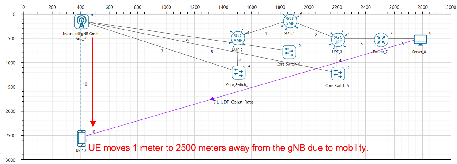
Effect of UE distance on throughput in FR1 and FR2
In this example we understand how the downlink UDP throughput of a UE varies as its distance from a gNB is increased. Open NetSim, Select Examples \(\rightarrow\) 5G NR \(\rightarrow\) Distance vs Throughput then click on the tile in the middle panel to load the example as shown in below screenshot.

The following network diagram illustrates what the NetSim UI displays when you open the example configuration file.

Frequency Range - FR1
Settings done in example config file.
Set grid length as 2000m \(\times\) 1000m from grid setting property panel on the right. This needs to be done before any device is placed on the grid.
Set distance between gNB 9 and UE 10 as 100m.
Click on gNB and expand the property panel on right side go to Interface (5G RAN) PHYSICAL LAYER, set the following properties as shown below.
| Properties | |
|---|---|
| CA Type | Inter band CA |
| CA Configuration | CA_2DL_1UL_n39_n41 |
| Numerology | 2 |
| Channel Bandwidth | 40 MHz |
| Numerology | 2 |
| Channel Bandwidth | 100 MHz |
| MCS Table | QAM64LOWSE |
| CQI Table | TABLE3 |
| Pathloss Model | 3GPP TR 38.901-7.4.1 |
| Outdoor Scenario | Urban Macro |
| LOS NLOS Selection | User Defined |
| LOS Probability | 0 |
| Shadow Fading Model | None |
| Fast Fading Model | No Fading |
Set Tx Antenna Count and Rx Antenna Count in gNB as 2 and 2.
Set Tx Antenna Count and Rx Antenna Count in UE as 2 and 2.
Go to Application properties and set the following properties as shown below.
| Application Properties | |
|---|---|
| Source Id | 8 |
| Destination Id | 10 |
| QoS | UGS |
| Transport Protocol | UDP |
| Packet Size | 1460 Bytes |
| Inter Arrival time | 23 \(\mu\)s |
| Start Time | 1 s |
The LTENR Radio measurement log file must be enabled from the design window.
LTENR Radio measurement Log can be enabled by clicking on the icon in Configure Reports \(>\) Plots \(>\) Network Logs option as shown below.

Run Simulation for 2s, after simulation completes go to metrics window and note down throughput value from application metrics.
Go back to the scenario and change the distance between gNB and UE as 200, 300, 400, 500, 600, 700, 800, 900, and 1000m and note down throughput from the results window. The other parameters in table shown below can be noted down from the LTE NR Radio measurement logs.
Frequency Range - FR2
Settings done in example config file
Set grid length as 1000m \(\times\) 500m from grid setting property panel.
Set distance between gNB 9 and UE 10 as 50m.
Click on gNB and expand the property panel on right side go to Interface (5G RAN) PHYSICAL LAYER, set the following properties as shown below.
| Properties | |||
|---|---|---|---|
| Physical Layer Properties | |||
| CA Type | Intra Band Contiguous CA | ||
| CA Configuration | CA_n258G | ||
| Numerology | Channel Bandwidth (MHz) per carrier | Frequency Range | |
| CA1,CA2 | 3 | 400 | FR2 |
| Channel Model | |||
| Pathloss Model | 3GPP TR 38.901-7.4.1 | ||
| Shadow Fading Model | None | ||
| Fast Fading Model | No Fading | ||
| Outdoor Scenario | Urban macro | ||
| LOS NLOS Selection | User defined | ||
| LOS Probability | 0 | ||
| MCS Table | QAM256 | ||
| CQI Table | TABLE2 | ||
Set Tx Antenna Count and Rx Antenna Count in gNB as 2 and 2.
Set Tx Antenna Count and Rx Antenna Count in UE as 2 and 2.
Go to Application properties and set the following properties as shown below.
| Application Properties | |
|---|---|
| Source Id | 8 |
| Destination Id | 10 |
| QoS | UGS |
| Transport Protocol | UDP |
| Packet Size | 1460 Bytes |
| Inter Arrival time | 2\(\mu\)s |
| Start Time | 1s |
The LTENR Radio measurement log file can be enabled as per the information provided above in Step 7.
Run Simulation for 1.05s, after simulation completes go to results window and note down throughput value from application metrics.
Go back to the scenario and change the distance between gNB and UE as 50, 100, 150, and 200 and note down throughput from the results window. The other parameters in the table shown below can be noted down from the LTENR Radio Measurement log.csv.
Results
NOTE: Filter the CC ID to 1 in the LTENR Radio measurement log file and same values have been considered in the tables given below. (SNR and CQI are shown for downlink Layer1).
Increase in distance leads to an increase in pathloss, which in turn hence leads to lower received power (and lower SNR). The lower SNR leads to a lower MCS, in turn a lower CQI and thereby results in lower throughputs. The drop for FR2 happens at a much faster rate in comparison to FR1. Note that the number of information bits is obtained from the Transport Block Size Determination calculations given in 3.9.15. The throughput would depend on the TBS.
Impact of MAC Scheduling algorithms on throughput, in a multi-UE scenario
In this example we understand how the scheduling algorithm affects the UDP download throughput of a multi-user (UE) system where the UEs are at different distances from the gNB. Open NetSim, Select Examples \(\rightarrow\) 5G NR \(\rightarrow\) Scheduling then click on the tile in the middle panel to load the example as shown in below screenshot

Multi UE throughput with UEs at different distances and channel is not time varying.
The following network diagram illustrates what the NetSim UI displays when you open this example configuration file.

Configuring the scheduling algorithm, and parameter settings in example config files
Set grid length as 12000m \(\times\) 6000m from grid property panel on the right.
Set distance as follows.
gNB 9 to UE 10 = 1500m
gNB 9 to UE 11 = 2000m, and
gNB 9 to UE 12 = 2500m
Go to gNB properties \(\rightarrow\) Interface (5G RAN), set the following properties as shown below. In the first sample the scheduling type is set to Round Robin, in the second to Proportional fair, and in the third to Max throughput.
| Properties | |
|---|---|
| Scheduling Type | Varies: Proportional Fair, Max throughput, Round Robin |
| CA type | Single Band |
| CA Configuration | n78 |
| Numerology | 1 |
| Channel Bandwidth | 100 MHz |
| Pathloss Model | 3GPP TR 38.901-7.4.1 |
| Outdoor Scenario | Urban macro |
| LOS NLOS Selection | User defined |
| LOS Probability | 1 |
| Shadow Fading Model | None |
| Fast Fading Model | No Fading |
Set Tx Antenna Count as 1 and Rx Antenna Count as 1 in gNB properties.
Set Tx Antenna Count as 1 and Rx Antenna Count as 1 in all the UEs.
Go to the Set Traffic tab in the top ribbon and create a CBR application as shown in the table below. To change the transport protocol, QoS, and IAT, click on the application and change the properties in the right-side property panel.
| Application Properties | Application 1 | Application 2 | Application 3 |
|---|---|---|---|
| Application Type | CBR | CBR | CBR |
| Source ID | 8 | 8 | 8 |
| Destination ID | 10 | 11 | 12 |
| QoS | UGS | UGS | UGS |
| Transport Protocol | UDP | UDP | UDP |
| Packet Size | 1460 Bytes | 1460 Bytes | 1460 Bytes |
| Inter-arrival time | 58.4 \(\mu\)s | 58.4 \(\mu\)s | 58.4 \(\mu\)s |
| Start Time | 1s | 1s | 1s |
Run Simulation for 10 s and note down throughput value in the results window in each sample. Recall that each sample has a different scheduling algorithm configured.
Results and discussions
The results with all the three UEs simultaneously downloading data is as given below.
| Scheduling | Application 1 | Application 2 | Application 3 | Aggregate |
|---|---|---|---|---|
| Round Robin | 64.65 | 37.22 | 19.59 | 121.46 |
| Proportional Fair | 64.65 | 37.23 | 19.59 | 121.46 |
| Max Throughput | 193.94 | 0.00 | 0.00 | 193.94 |

Next, consider a scenario with only one of the UEs seeing DL traffic (we don’t provide inbuilt configuration file for this, and since it is a simple exercise for a user) First, run for the UE at 1500m, then for UE at 2000m and finally for UE at 2500m. This gives the maximum achievable throughput per node since the gNB resources (bandwidth) is not shared between 3 UEs and is fully dedicated to just one UE. The results are below.
| Distance from gNB (m) | Application ID | Throughput (Mbps) | Remarks |
|---|---|---|---|
| 1500 | 1 | 193.94 | UE 1 alone has full buffer DL traffic |
| 2000 | 2 | 111.66 | UE 2 alone has full buffer DL traffic |
| 2500 | 3 | 49.95 | UE 3 alone has full buffer DL traffic |
The PHY rate is decided per the received SNR. Therefore, a UE closer to the gNB will get a higher data rate than a UE further away. In this example the distances from the gNB are such that UE12 Distance \(>\) UE11 Distance \(>\) UE10 Distance.
In Round Robin PRBs are allocated equally among all three nodes. However, throughputs are in the order UE10 Distance \(>\) UE11 Distance \(>\) UE12 Distance because of their distances from the gNB. The individual throughputs seen by each of the UEs is exactly \(\frac{1}{3}\) of the throughput as shown in Table 4-17. The PF scheduler results will match that of the RR scheduler since the channel is not time varying. In Max throughput scheduling the PRBs are allocated such that the system gets the maximum download throughput. The nearest UE will get all the resources and its throughput will be \(3\) times the throughput of the UE which got the max throughput in RR.
Multi UEs at different distances with a time varying channel
Configuring the scheduling algorithm, and parameter settings will remain the same for the case below.
Changes in the gNB properties are as follows.
Click on gNB and go to Interface (5G RAN), set the following properties as shown below. In the first sample the scheduling type is set to Round Robin, in the second to Proportional fair, and in the third to Max throughput.
| Properties | |
|---|---|
| Scheduling Type | Varies: Proportional Fair, Max throughput, Round Robin |
| CA Type | Single Band |
| CA Configuration | n78 |
| Numerology | 1 |
| Channel Bandwidth | 100 MHz |
| Pathloss Model | 3GPP TR 38.901-7.4.1 |
| Outdoor Scenario | Urban Macro |
| LOS NLOS Selection | User Defined |
| LOS Probability | 1 |
| Fast Fading Model | Rayleigh |
| MIMO Beamforming Model | Eigen |
Run Simulation for 10s and note down throughput value in the results window in each sample.
Enable EWMA MAC throughput plot

Results and discussions
The results with all the three UEs simultaneously downloading data are as given below.
| Scheduling | Application 1 | Application 2 | Application 3 | Aggregate |
|---|---|---|---|---|
| Round Robin | 51.58 | 30.06 | 18.34 | 100.00 |
| Proportional Fair | 69.82 | 41.95 | 24.73 | 135.50 |
| Max Throughput | 139.84 | 28.19 | 5.32 | 173.35 |
While running the Proportional fair sample enable Application throughput vs time and EWMA MAC throughput plot to observe the throughput differences.

A difference in the performance of the RR and PF schedulers can be seen when the channel is time varying (of the order of the coherence time which is 10ms). To induce time varying randomness in the channel we enable fading and beamforming. Thus, after every 10ms, NetSim draws an i.e. fading random variable, as the additional loss. Under these conditions, the RR scheduler would allot resources to the UEs in a round robin fashion, whereas the PF scheduler would give preference to the UE which sees the best channel (highest SINR). The reason why the RR scheduler yields lower throughputs than the PF scheduler is that the RR scheduler is not “opportunistic,” i.e., it does not take advantage of the knowledge that a UE has a good channel in the next slot and continues to serve the UEs cyclically. The results are shown in Table 4-19; observe how this is different from Table 4-17 where the channel is not time varying.

In the earlier results we observed the average (overtime) throughput while in Figure 4-25 we observed the MAC throughput vs Time for all 3 UEs. Key points are:
Channel Coherence Time: The wireless channel fading gain changes at this time scale, causing fluctuations in the signal quality and, consequently, the achievable throughput.
Proportional Fair Scheduler Behavior: The Proportional Fair (PF) scheduling algorithm aims to balance fairness and throughput by allocating resources to users based on their current channel quality relative to their average throughput
This dynamic allocation process leads to throughput variations as the scheduler continuously adjusts resource assignments to maintain fairness while exploiting favorable channel conditions. Thus, when a user experiences good channel conditions relative to their average, they receive more resources, leading to increased throughput. Conversely, when channel conditions degrade or other users are prioritized, a user’s throughput will decrease. The MAC throughput would be higher than the application throughput because of the overheads of the various layers.
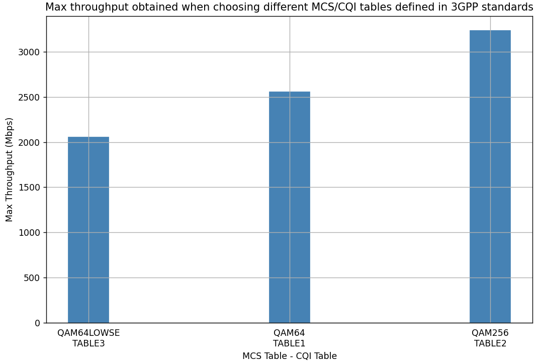
Max Throughput for different MCS and CQI
Open NetSim, Select Examples \(\rightarrow\) 5G NR \(\rightarrow\) Max Throughput vs MCS and CQI then click on the tile in the middle panel to load the example as shown in below screenshot.

The following network diagram illustrates what the NetSim UI displays when you open the example configuration file.

Settings done in example config file:
Set grid length as 500m \(\times\) 250m from grid property panel.
Go to gNB properties \(\rightarrow\) Interface (5G RAN), set the following properties as shown below.
| Properties | |||
|---|---|---|---|
| Physical Layer Properties | |||
| CA TYPE | Intra Band Contiguous CA | ||
| CA Configuration | CA n258G | ||
| Numerology | Channel Bandwidth (MHz) | Frequency Range | |
| CA1 | 3 | 400 | FR2 |
| CA2 | 3 | 400 | FR2 |
| Pathloss Model | None | ||
Go to Application properties and set the following properties as shown below.
| Application Properties | |
|---|---|
| Source Id | 8 |
| Destination Id | 10 |
| Transport Protocol | UDP |
| Start Time | 1 s |
| Packet Size | 1460 Bytes |
| Inter Arrival time | 1 \(\mu\)s |
| Generation Rate | 11680 Mbps |
Set Tx Antenna Count as 2 and Rx Antenna Count as 1 in gNB properties.
Set Tx Antenna Count as 1 and Rx Antenna Count as 2 in UE properties.
Run Simulation for 1.002s, after simulation completes go to results window and note down throughput and delay value from application metrics.
For this Scenario set MCS Table as QAM64LOWSE and CQI Table as TABLE3 and note down throughput.
Go Back to the Scenario and set MCS Table as QAM64 and CQI Table as TABLE1 and note down throughput.
Go Back to the Scenario and set MCS Table as QAM256 and CQI Table as TABLE2 and note down throughput.
Result:
| MCS Table | CQI Table | Throughput (Mbps) |
|---|---|---|
| QAM64LOWSE | TABLE3 | 2084.88 |
| QAM64 | TABLE1 | 2633.84 |
| QAM256 | TABLE2 | 3439.76 |
Load balancing in 5G using Cell Individual Offset (CIO)
Introduction
Overview
Mobility load balancing is a 3GPP Release 17 AI/ML for NG RAN Use Case. It involves transferring load from overloaded cells to under-loaded neighboring cells, for optimizing network performance and user experience. This study describes the network setup, presents the simulation results before and after applying CIO-based load balancing, and discusses the observed outcomes.
Concept
Default Association: The default user equipment (UE) association with a base station is based on Maximum signal strength.
Load Balancing Goal: Modify the association/handover criteria to distribute network load efficiently across available cells.
Role of Cell Individual Offset (CIO)
Cell Individual Offset (CIO) is a configurable parameter used to artificially modify the signal quality measurement of a target cell during the handover evaluation process. In NetSim, the CIO value is added to the measured SINR of the candidate cell.
\[\begin{equation} SINR_{eff} = SINR_{actual} + CIO \end{equation}\]
A positive CIO increases the effective signal value.
A negative CIO decreases the effective signal value.
CIO is typically applied to control handovers and implement load balancing across cells.
Network Setup

Network Settings
Environment size is set to 600m \(\times\) 500m
Consider three Macro cell gNB sector antennas and 500 UEs spread across the network grid such that
75 UEs are located near the gNBs (represented in green)
125 UEs are located near at the cell center (represented in yellow)
300 UEs are located at the cell edge. (represented in red)
The 3 gNBs (with sector antennas) are co-located at the top left with \(120^\circ\).
gNB 1 operates in the n50 (1.5 GHz band)
gNB 2 operates in the n38 (2.6 GHz band)
gNB 3 operates in the n78 (3.5 GHz band)
The gNB properties and the Traffic model properties are set as follows:
| System Model and Parameters | |
|---|---|
| No of gNBs | 3 (3 sector carriers) |
| No of UEs | 500 |
| Band | n78, n50, n38 |
| Numerology | 1 |
| Channel Bandwidth (MHz) | 40 |
| Antenna | 4T4R |
| Pathloss model | Log Distance |
| Pathloss Exponent (\(\eta\)) | 3.8 |
| Shadowing Model | Log Normal |
| Standard Deviation (dB) | 5 |
| Simulation Time (s) | 10 |
| Traffic Type | Custom |
| Traffic generation rate | 467.2 Kbps |
| Packet size | 1460B |
| Inter packet arrival time | 25000 \(\mu\)s (Exponential) |
Set the Cell Individual Offset present under Interface (RAN) \(>\) Datalink Layer \(>\) Handover \(>\) Cell Individual Offset as follows:
gNB1 1475 MHz: \(-4.77\) dB
gNB2 2595 MHz: 0 dB
gNB3 3550 MHz: 4.77 dB.
These negative CIO value shifts the load away from gNB1; the positive CIO value shifts the load towards gNB3.
Enable PRB Utilization vs time Plots and Radio resource allocation log
Run the simulation for 10 seconds.
Results
After simulation, plot the PRB Utilization for the three gNBs i.e., gNB1 1475MHz, gNB2 2595MHz, gNB3 3550MHz with CIO and without CIO.
PRB Utilization vs time plot without CIO (default configuration)

PRB Utilization vs time plot with CIO enabled

Discussion
These graphs show resource (PRB) usage of different 5G base stations over time, comparing scenarios with and without load balancing.
Without load balancing (Figure 4-30): Base station 1 (gNB1_1475MHz) is overloaded at \(\sim\)100% while gNB2 (2575 MHz) and gNB3 (3550 MHz) are underused and operating around 30% and 25% PRB utilization respectively.
With load balancing (Figure 4-31): Resource usage is more evenly distributed across all base stations, with gNB1 around 60–70% and other gNBs operating at 30–40%.
We can observe the association of UEs with gNBs before and after load balancing.
To analyze this, we use the LTENRRadioMeasurementsLog.csv and DeviceList.xlsx files.
A Python script reads the UE association entries at two time points—initial and post-load balancing—and generates corresponding plots.

| gNB | Count of Associated UEs |
|---|---|
| gNB1 1475 MHz | 321 |
| gNB2 2595 MHz | 122 |
| gNB3 3550 MHz | 57 |
| Total | 500 |
| gNB | Count of Associated UEs |
|---|---|
| gNB1 1475 MHz | 192 |
| gNB2 2595 MHz | 105 |
| gNB3 3550 MHz | 203 |
| Total | 500 |
Python code for data analysis and visualization
import pandas as pd
import matplotlib.pyplot as plt
import numpy as np
import sys
import os

def get_color_map():
    return {
        'GNB1_1475MHZ': '#228B22',  # Green
        'GNB2_2595MHZ': '#FFD700',  # Yellow
        'GNB3_3550MHZ': '#d62728'   # Red
    }

def plot_combined_association(log_df, device_list_df, output_dir):
    snapshots = {
        161.5: 'UE-gNB Initial Association',
        220: 'UE-gNB Association After Load Balancing'
    }
    fig, axs = plt.subplots(1, 2, figsize=(14, 6), sharex=True, sharey=True)
    color_map = get_color_map()
    gnb_names = list(color_map.keys())

    all_x = device_list_df['X Pos/LON']
    all_y = device_list_df['Y Pos/LAT']
    x_min, x_max = all_x.min() - 20, all_x.max() + 20
    y_min, y_max = all_y.min() - 20, all_y.max() + 20

    for ax, (time_snapshot, title) in zip(axs, snapshots.items()):
        filtered_df = log_df[(log_df['Time(ms)'] == time_snapshot) &
                             (log_df['Channel'] == 'PDSCH') &
                             (log_df['isAssociated'] == True)]

        merged_df = pd.merge(filtered_df, device_list_df, how='left',
                             left_on='UE Name', right_on='Device Name')

        for gnb in gnb_names:
            ue_group = merged_df[merged_df['gNB or eNB Name'] == gnb]
            ax.scatter(ue_group['X Pos/LON'], ue_group['Y Pos/LAT'],
                       label=f'{gnb} UEs', s=30, marker='o',
                       color=color_map[gnb])

        gnb_data = device_list_df[
            device_list_df['Device Type'].str.contains('gNB')]
        for _, gnb in gnb_data.iterrows():
            ax.scatter(gnb['X Pos/LON'], gnb['Y Pos/LAT'],
                       label=gnb['Device Name'], s=70, marker='^',
                       color='black')

        ax.set_title(title, fontweight='bold', fontsize=12, pad=10)
        ax.set_xlabel('X Coordinate', fontsize=10)
        ax.set_xlim(x_min, x_max)
        ax.set_ylim(y_max, y_min)
        ax.grid(True, linestyle='--', linewidth=0.5)

    axs[0].set_ylabel('Y Coordinate', fontsize=10)
    handles, labels = axs[1].get_legend_handles_labels()
    fig.legend(handles, labels, loc='lower center',
               fontsize=14, ncol=3, markerscale=2)
    plt.tight_layout(rect=[0, 0.08, 1, 1])
    output_path = os.path.join(output_dir,
                               'combined_association_plot.png')
    plt.savefig(output_path, dpi=300)
    plt.close()
    print(f"Combined plot saved: {output_path}")

if __name__ == '__main__':
    if len(sys.argv) != 4:
        print("Usage: python combined_association.py "
              "<log_csv_path> <device_list_excel_path> "
              "<output_directory>")
        sys.exit(1)

    log_path = sys.argv[1]
    device_path = sys.argv[2]
    output_dir = sys.argv[3]

    log_df = pd.read_csv(log_path)
    device_df = pd.read_excel(device_path)
    plot_combined_association(log_df, device_df, output_dir)
4G vs. 5G: Capacity analysis for video downloads
Open NetSim, Select Examples \(\rightarrow\) 5G NR \(\rightarrow\) 4G vs 5G then click on the tile in the middle panel to load the example as shown in below screenshot.

4G
Under 4G click on 40 Nodes Sample, the following network diagram illustrates what the NetSim UI displays when you open the example configuration file.

Settings done in example config file:
Set grid length as 3300\(\times\)5200m from grid property panel on the right.
Set the following property as shown in below given Table.
| eNB Properties \(\rightarrow\) Interface (LTE) | |||||||
|---|---|---|---|---|---|---|---|
| CA | Freq. Range | DL UL Ratio | Numerology | Channel BW | |||
| CA Type | Intra Band Non-Contiguous CA | ||||||
| CA Configuration | CA_4DL_42C_42C_2UL_42C_BCS1 | ||||||
| CA1 | FR1 | 1:1 | 0 | 20 MHz | |||
| CA2 | FR1 | 1:1 | 0 | 20 MHz | |||
| CA3 | FR1 | 1:0 | 0 | 20 MHz | |||
| CA4 | FR1 | 1:0 | 0 | 20 MHz | |||
| PDSCH and PUSCH Configuration | |||||||
| MCS Table | QAM64 | ||||||
| CSI Report Configuration | |||||||
| CQI Table | TABLE1 | ||||||
| Channel Model | |||||||
| Pathloss Model | None | ||||||
Frequency range FR1, Numerology = 0, Bandwidth = 20 MHz with QAM 64 MCS table represents a 4G configuration.
Set Uplink speed and Downlink speed as 10000 Mbps and BER as 0 in all wired links.
Set Tx Antenna Count as 2 and Rx Antenna Count as 1 in eNB \(>\) Interface LTE \(>\) Physical Layer.
Set Tx Antenna Count as 1 and Rx Antenna Count as 2 in UE \(>\) Interface LTE \(>\) Physical Layer.
Configure 40 applications with Source id as 3 and Destination id as 5, 6, 7, 8, 9, 10, 11, 12, 13, 14, 15, 16, 17, 18, 19, 20, 21, 22, 23, 24, 25, 26, 27, 28, 29, 30, 31, 32, 33, 34, 35, 36, 37, 38, 39, 40, 41, 42, 43 and 44 and set the properties as shown below. This would generate 2.5 Mbps of traffic per user. Transport Protocol is set to UDP in all the applications.
| Application Properties | |
|---|---|
| Frame Per Sec | 50 |
| Pixel Per Frame | 50000 |
| Mu | 1 |
| Start Time | 1s |
Run simulation for 2 sec. After simulation completes go to results window and note down throughput and delay value from application metrics.
Increase the number of UE’s and number of applications as 40, 80, 120, 160, 200, 240 and 280 and note down throughput and delay value from application metrics.
5G
Under 5G click on 40 Nodes Sample, the following network diagram illustrates what the NetSim UI displays when you open the example configuration file.

Settings done in example config file:
For the above 5G scenario set the following given properties.
The Tx Antenna Count was set to 2 and Rx Antenna Count was set to 1 in gNB \(>\) Interface 5G RAN \(>\) Physical Layer.
The Tx Antenna Count was set to 1 and Rx Antenna Count was set to 2 in UE \(>\) Interface 5G RAN \(>\) Physical Layer.
Frequency range FR2, Numerology = 3, Bandwidth = 400 MHz with QAM 256 MCS table represent a 5G configuration
The Uplink and Downlink speed was set to 10000 Mbps and BER as 0 in wired links.
Run simulation for 2 sec. After simulation completes go to results window and note down throughput and delay value from application metrics.
Increase number of UE’s and number of applications as 40, 80, 120, 160, 200, 240 and 280 and note down throughput and delay value from application metrics.
\[\begin{equation} Throughput\ Per\ User\ (Mbps) = \frac{Sum\ of\ throughputs\ (Mbps)}{Number\ of\ User} \end{equation}\]
\[\begin{equation} Delay\ Per\ User\ (\mu s) = \frac{Sum\ of\ Delays\ (\mu s)}{Number\ of\ User} \end{equation}\]
Theoretical PHY Rate Calculation
The 4G/5G PHY data rate is given by the expression
\(PHY\ data\ rate(in\ Mbps) = 10^{-6} \sum_{j=1}^{J} (v_{Layers}^{(j)}) \cdot Q_m^{(j)} \cdot f^{(j)} \cdot R \frac{N_{PRB}^{BW(j),\mu} \cdot 12}{T_s^{\mu}} (1 - OH^{(j)})\),
where \(T_s^{\mu} = \frac{10^{-3}}{14 \cdot 2^{\mu}}\)
This expression gives the PHY rate; the application throughput would be lower than the PHY rate given the overheads in the various layers.
4G:
Number of carriers: 4, Number of layers = \(\min(N_t\ (gNB),\ N_r(UE)) = \min(2, 2) = 2\), Numerology: 0. The BW per carrier is 20 MHz, with each carrier having 100 PRBs. In this experiment settings the DL:UL Ratio is 1:1 for 2 carriers and 1:0 for 2 carriers. Avg DL:UL ratio is 3:1 and hence the DL fraction = \(\frac{3}{3+1} = \frac{3}{4}\).
Applying the 4G PHY data rate formula
\[\begin{equation} PHY\ Rate = 10^{-6}\left(2 \times 6 \times 1 \times \frac{948}{1024} \times \frac{100 \times 12}{\left(\frac{10^{-3}}{14 \cdot 2^{0}}\right)} \times (1 - 0.25)\right) \times 4 = 559.40\ \text{Mbps} \end{equation}\]
Where \(4\) is the number of carriers
Multiplying by the DL fraction we obtain the downlink PHY rate as \(559.40 \times \frac{3}{4}\) = \(419.93\) Mbps
5G:
Number of carriers: 4, Number of layers = \(\min(N_t\ (gNB),\ N_r(UE)) = \min(2, 2) = 2\), Numerology: 3. The BW per carrier is 400 MHz with each carrier having 264 PRBs. In this experiment settings, the DL:UL Ratio: 1:1 for both carriers
Applying the 5G PHY data rate formula, we get
\[\begin{equation} PHY\ Rate = 10^{-6}\left(2 \times 8 \times 1 \times \frac{948}{1024} \times \frac{264 \times 12}{\left(\frac{10^{-3}}{14 \cdot 2^{3}}\right)} \times (1 - 0.18)\right) \times 2 = 7568.22\ \text{Mbps} \end{equation}\]
Where \(2\) is the number of carriers
Multiplying by the DL fraction we obtain the downlink PHY rate as \(7568.22 \times \frac{1}{2} = 3784.11\) Mbps.
We vary the UE count from 40 to 280 in steps of 40. Each UE is downloading video at a rate of 2.5 Mbps. Post simulation, we plot the throughput per UE for 4G and 5G as the UE count is increased from 40 to 280.
Results:
| 4G (Devices downloading video) | 5G (Devices downloading video) | |||||
|---|---|---|---|---|---|---|
| Users | Per user (Mbps) | Agg. (Mbps) | Avg delay (\(\mu\)s) | Per user (Mbps) | Agg. (Mbps) | Avg delay (\(\mu\)s) |
| 40 | 2.43 | 97.23 | 3113.92 | 2.45 | 98.08 | 392.12 |
| 80 | 2.44 | 195.41 | 5539.42 | 2.44 | 195.69 | 649.40 |
| 120 | 2.44 | 293.13 | 7965.39 | 2.44 | 293.29 | 908.43 |
| 160 | 2.41 | 386.24 | 10177.97 | 2.45 | 392.18 | 1171.72 |
| 200 | 2.06 | 412.68 | 82788.13 | 2.44 | 489.94 | 1430.69 |
| 240 | 1.71 | 412.53 | 152792.20 | 2.44 | 587.86 | 1689.47 |
| 280 | 1.47 | 412.31 | 202942.80 | 2.44 | 685.70 | 1946.88 |
In the earlier section, we had predicted a PHY rate of 419 Mbps. We observe that the aggregate application throughput of 4G saturates at 407 Mbps. The \(\approx 10\%\) difference is due to the overheads in the various layers. The required rate for each video application is \(\approx 2.5\) Mbps and we see that 4G is able to support full rate for upto 160 UEs. At 200 UEs the capacity required is \(\approx 200 \times 2.5 = 500\) Mbps which is more than what is available. Therefore, the rate per user starts decreasing for UE counts of 200, 240 and 280. In line with this, we see that the average delay increases exponentially from 200 UEs onwards.
On the other hand, 5G can handle a PHY rate of \(3784\) Mbps or \(\approx 3400\) Mbps of application throughput. Thus, we see that 5G is easily able to provide full rate of \(\approx 2.5\) Mbps to each UE even when the total UE count is 280.
Throughput per user vs. Number of users for 4G and for 5G

Average delay vs. Number of users for 4G and for 5G

5G-Peak-Throughput
Open NetSim, Select Examples \(\rightarrow\) 5G NR \(\rightarrow\) 5G Peak Throughput then click on the tile in the middle panel to load the example as shown in below screenshot

3.5 GHz n78 band
The following network diagram illustrates what the NetSim UI displays on clicking.

Settings done in example config file:
Set the following property as shown in below given Table.
| gNB Properties \(\rightarrow\) Interface (5G RAN) | |
|---|---|
| CA Type | Single Band |
| CA Configuration | n78 |
| Frequency Range | FR1 |
| DL/UL Ratio | 4:1 |
| Numerology | 2 |
| Channel Bandwidth | 50 MHz |
| MCS Table | QAM256 |
| CQI Table | TABLE2 |
| Pathloss Model | None |
The Tx Antenna Count was set to 8 and Rx Antenna Count was set to 4 in gNB \(>\) Interface 5G RAN \(>\) Physical Layer.
The Tx Antenna Count was set to 4 and Rx Antenna Count was set to 8 in UE \(>\) Interface 5G RAN \(>\) Physical Layer.
Set 2 applications Downlink source node as 8, and destination node as 10, Uplink source node as 10, and destination node as 8. Transport Protocol is set to UDP in all the applications.
| Application Properties | |
|---|---|
| Start Time (s) | 1 |
| Packet Size (Byte) | 1460 |
| Inter Arrival Time (\(\mu\)s) | 2.92 |
| Start Time (s) | 1 |
| Packet Size (Byte) | 1460 |
| Inter Arrival Time (\(\mu\)s) | 5.84 |
Enable the Throughput vs time plot under Application and link and run simulation for 1.1 sec. After simulation completes go to results window and note down throughput value from application metrics.
Go back to the Scenario and change channel bandwidth to 100 MHz, run simulation for 1.1 sec and note down throughput value from application metrics.
Result:
| Bandwidth (MHz) | Throughput (Mbps) CBR UDP UL | Throughput (Mbps) CBR UDP DL |
|---|---|---|
| 50 | 128.71 | 1597.47 |
| 100 | 270.62 | 3366.87 |

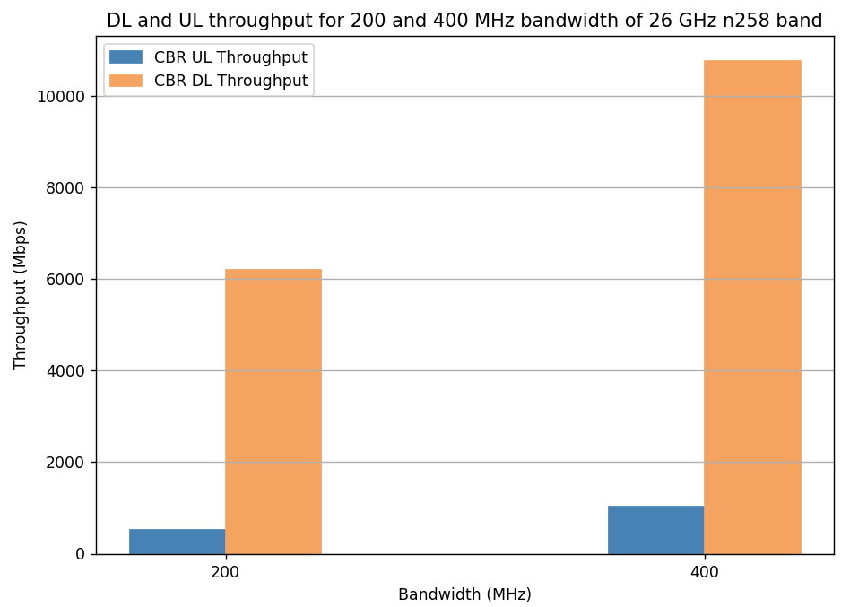
26 GHz n258 band
The following network diagram illustrates what the NetSim UI displays on clicking.

Settings done in example config file:
Set the following property as shown in below Table.
| gNB Properties \(\rightarrow\) Interface (5G RAN) | |
|---|---|
| CA Type | Single Band |
| CA Configuration | n258 |
| DL/UL Ratio | 4:1 |
| Frequency Range | FR2 |
| Numerology | 3 |
| Channel Bandwidth | 200 MHz |
| MCS Table | QAM256 |
| CQI Table | TABLE2 |
| Pathloss Model | None |
The Tx Antenna Count was set to 8 and Rx Antenna Count was set to 4 in gNB \(>\) Interface 5G RAN \(>\) Physical Layer.
The Tx Antenna Count was set to 4 and Rx Antenna Count was set to 8 in UE \(>\) Interface 5G RAN \(>\) Physical Layer.
Set 2 applications Downlink source node as 8 destination node as 10, Uplink source node as 10 destination node as 8. Transport Protocol is set to UDP in all the applications.
| Application Properties | |
|---|---|
| Start Time (s) | 1 |
| Packet Size (Byte) | 1460 |
| Inter Arrival Time (\(\mu\)s) | 1 |
| Start Time (s) | 1 |
| Packet Size (Byte) | 1460 |
| Inter Arrival Time (\(\mu\)s) | 4 |
After simulation completes go to results window and note down throughput value from application metrics.
Go back to the Scenario and change channel bandwidth to 400 MHz, run simulation for 1.1 sec and note down throughput value from application metrics.
Result:
| Bandwidth (MHz) | Throughput (Mbps) CBR UDP UL | Throughput (Mbps) CBR UDP DL |
|---|---|---|
| 200 | 518.35 | 6283.72 |
| 400 | 1041.15 | 11648.46 |
Impact of distance on throughput for n261 band in LOS and NLOS states
Objective: We observe throughput of a UE (operating in the n261 band with a channel bandwidth of 100 MHz), moving away from the gNB from 1 m to 3.5 Km. The variation of throughput is plotted in both LOS and NLOS states. Since 5G simulations take a long time to complete, and given our goal of studying throughput vs. distance, we have set an unrealistic speed of 20 m every 10 ms to complete the UE movement in a short time duration.
Open NetSim, Select Examples \(\rightarrow\) 5G NR \(\rightarrow\) Distance vs Throughput n261 band then click on the tile in the middle panel to load the example as shown in below Figure.

NetSim UI displays the configuration file corresponding to this experiment as shown below.

DL: UL Ratio 4:1
LOS and NLOS
The following settings were done to generate this sample:
Step 1: A network scenario is designed in NetSim GUI consisting of 1 gNB, 5G-Core, and 1 UE and 1 Router and 1 Wired Node in the “5G NR” Network Library.
Step 2: Grid length was set to 8000 m \(\times\) 4000 m.
Step 3: The device positions are set as per the table given below.
| Device | UE_10 | gNB_9 |
|---|---|---|
| x-axis | 500 | 500 |
| y-axis | 1 | 0 |
Step 4: The following properties were set in Interface (5G RAN) of gNB
| Parameter | Value |
|---|---|
| Tx Power | 40 |
| gNB Height | 10 m |
| CA Type | Single Band |
| CA Configuration | n261 |
| Component Carrier 1 | |
| DL-UL Ratio | 4:1 |
| Numerology | 3 |
| Channel Bandwidth | 100 MHz |
| PDSCH and PUSCH Configuration | |
| MCS Table | QAM64LOWSE |
| CSI Report Configuration | |
| CQI Table | TABLE3 |
| Channel Model | |
| Pathloss Model | 3GPP TR 38.901-7.4.1 |
| Outdoor Scenario | Urban Macro |
| LOS NLOS Selection | User Defined |
| LOS Probability | 1 |
| Shadow Fading Model | None |
| Fast Fading Model | No Fading |
Step 5: Set Tx Antenna Count and Rx Antenna Count as 2 and 2 in gNB properties \(>\) Interface(5G RAN) \(>\) Physical Layer.
Step 6: Set Tx Antenna Count and Rx Antenna Count as 2 and 2 in UE properties \(>\) Interface(5G RAN) \(>\) Physical Layer.
Step 7: Two CBR Applications were generated from between the Server 8 and UE 10 with the following values.
| Parameter | Value |
|---|---|
| APP1 CBR DL | |
| Source | Server 8 |
| Destination | UE 10 |
| Start Time (s) | 1 |
| Packet Size (Bytes) | 1460 |
| IAT (\(\mu\)s) | 11.68 |
| Generation Rate (Mbps) | 1000 |
| Transport Protocol | UDP |
| APP2 CBR UL | |
| Source | UE 10 |
| Destination | Server 8 |
| Start Time (s) | 1 |
| Packet Size (Bytes) | 1460 |
| IAT (\(\mu\)s) | 97.33 |
| Generation Rate (Mbps) | 120 |
| Transport Protocol | UDP |
Step 8: In the Device Position Properties of UE 10, set Mobility Model as File Based Mobility
File Based Mobility: In File Based Mobility, users can write their own custom mobility models and define the movement of mobile users. Create a mobility.csv file for UE’s involved in mobility with each step equal to 4 sec with distance 100 m. The NetSim Mobility File (mobility.csv) format is as follows:
| #Time(s) | Device ID | X | Y | Z |
|---|---|---|---|---|
| 1 | 10 | 500 | 50 | 0 |
| 1.01 | 10 | 500 | 70 | 0 |
| 1.02 | 10 | 500 | 90 | 0 |
| 1.03 | 10 | 500 | 110 | 0 |
| . | . | . | . | . |
| 2.65 | 10 | 500 | 3350 | 0 |
| 2.66 | 10 | 500 | 3370 | 0 |
| 2.67 | 10 | 500 | 3390 | 0 |
| 2.68 | 10 | 500 | 3410 | 0 |
| 2.69 | 10 | 500 | 3430 | 0 |
| 2.7 | 10 | 500 | 3450 | 0 |
| 2.71 | 10 | 500 | 3470 | 0 |
| 2.72 | 10 | 500 | 3490 | 0 |
| 2.73 | 10 | 500 | 3510 | 0 |
Step 9: Enable application throughput vs time plot under Plots tab in the NetSim GUI.
Step 10: Run simulation for 2.75 s.
Step 11: Similarly, in LOS, set the LOS Probability to 0 in gNB properties and simulate the scenario for 2.75 s.
Results:
Downlink Line-of-Sight (LOS) and Non-Line-of-Sight (NLOS) Plots


Uplink Line-of-Sight (LOS) and Non-Line-of-Sight (NLOS) Plots


Discussion: The downlink throughput of 478.1 Mbps is maintained till \({\sim}450\) m in LOS whereas, it is maintained till 150 m in NLOS. Similarly, the uplink throughput of 114 Mbps is maintained till 150 m in LOS whereas, it is maintained till 130 m in NLOS. The Uplink throughput falls to the lowest level at \({\sim}750\) m in LOS and at \({\sim}150\) m in NLOS.
DL: UL Ratio 3:2
LOS and NLOS
Step 1: All the properties were set as in DL: UL-Ratio 4:1.
Step 2: In the gNB properties \(\rightarrow\) Interface 5G RAN, the DL:UL ratio was set to 3:2.
Step 3: The following settings were done in application properties:
| Parameter | Value |
|---|---|
| APP1 CBR DL | |
| Source | Server 8 |
| Destination | UE 10 |
| Start Time (s) | 1 |
| Packet Size (Bytes) | 1460 |
| IAT (\(\mu\)s) | 11.68 |
| Generation Rate (Mbps) | 1000 |
| Transport Protocol | UDP |
| APP2 CBR UL | |
| Source | UE 10 |
| Destination | Server 8 |
| Start Time (s) | 1 |
| Packet Size (Bytes) | 1460 |
| IAT (\(\mu\)s) | 38.93 |
| Generation Rate (Mbps) | 300 |
| Transport Protocol | UDP |
Step 3: Run simulation for 2.75 s.
Step 4: Similarly, in LOS, set the LOS Probability to 0 in gNB properties and run simulation for 2.75 s.
Results:
Downlink Line-of-Sight (LOS) and Non-Line-of-Sight (NLOS) Plots


Uplink Line-of-Sight (LOS) and Non-Line-of-Sight (NLOS) Plots


Inference: The downlink throughput of 359.74 Mbps is maintained till \({\sim}550\) m in LOS whereas, it is maintained till 150 m in NLOS. Similarly, the uplink throughput of 120 Mbps is maintained till 170 m in LOS whereas, it is 35.97 Mbps maintained till 130 m in NLOS. The Uplink throughput falls to the lowest level at \({\sim}750\) m in LOS and at \({\sim}150\) m in NLOS.
gNB cell radius for different data rates
Open NetSim, Select Examples \(\rightarrow\) 5G NR \(\rightarrow\) gNB cell radius for different data rates then click on the tile in the middle panel to load the example as shown in below screenshot

3.5 GHz n78 urban gNB cell radius for different data rates
The following network diagram illustrates what the NetSim UI displays on clicking.

Setting done in example config file:
Set the following property as shown in below Table.
| gNB Properties \(\rightarrow\) Interface (5G RAN) | |
|---|---|
| Property | Value |
| gNB Height | 10 m |
| Tx Power | 40 |
| CA Type | Single Band |
| CA Configuration | n78 |
| Component Carrier 1 | |
| DL: UL | 4:1 |
| Numerology | 2 |
| Channel Bandwidth | 50 MHz |
| PDSCH and PUSCH Configuration | |
| MCS Table | QAM256 |
| CSI Report Configuration | |
| CQI Table | TABLE2 |
| Channel Model | |
| Pathloss Model | 3GPP TR 38.901-7.4.1 |
| Outdoor Scenario | Urban Macro |
| LOS NLOS Selection | 3GPP TR 38.901-Table7.4.2-1 |
| Shadow Fading Model | None |
| Fast Fading Model | No Fading |
Set the Tx Antenna Count as 8 and Rx Antenna Count as 1 in gNB \(>\) Interface 5G RAN \(>\) Physical Layer.
Set the Tx Antenna Count as 1 and Rx Antenna Count as 8 in UE \(>\) Interface 5G RAN \(>\) Physical Layer.
Set the following application properties:
| App_1_CBR | Value |
|---|---|
| Source Id | 8 |
| Destination Id | 10 |
| Packet Size | 1460 |
| IAT | 1.94 \(\mu\)s |
| Start time | 1 s |
| Transport Protocol | UDP |
| Generation Rate | 6 Gbps |
Run simulation for 1.1 sec. After simulation completes go to results window and note down throughput value from application metrics.
Go back to the Scenario and change distance between gNB and UE to 100 m, 130 m, 150 m, 170 m, 190 m, 200 m, 300 m, 330 m, and 350 m and run simulation for 1.1 sec.
Result:
| Cell Radius (m) | Data Rate (Mbps). Downlink |
|---|---|
| 1500 Mbps Downlink | |
| 100 | 1597.47 |
| 130 | 1421.22 |
| 150 | 1278.02 |
| 1000 Mbps Downlink | |
| 170 | 1167.76 |
| 190 | 969.44 |
| 200 | 925.40 |
| 500 Mbps Downlink | |
| 300 | 506.79 |
| 330 | 418.61 |
| 350 | 374.57 |
26 GHz n258 urban gNB cell radius for different data rates
Setting done in example config file:
Set the following property as shown in below given table:
| gNB Properties \(\rightarrow\) Interface (5G RAN) | |
|---|---|
| Property | Value |
| gNB Height | 10 m |
| Tx Power | 40 |
| CA Type | Single Band |
| CA Configuration | n258 |
| Component Carrier 1 | |
| DL: UL | 4:1 |
| Numerology | 2 |
| Channel Bandwidth | 200 MHz |
| PDSCH and PUSCH Configuration | |
| MCS Table | QAM256 |
| CSI Report Configuration | |
| CQI Table | TABLE2 |
| Channel Model | |
| Pathloss Model | 3GPP TR 38.901-7.4.1 |
| Outdoor Scenario | Urban Macro |
| LOS_NLOS Selection | 3GPP TR 38.901-Table7.4.2-1 |
| Shadow Fading Model | None |
| Fast Fading Model | No Fading |
Set the Tx Antenna Count as 8 and Rx Antenna Count as 1 in gNB \(>\) Interface 5G RAN \(>\) Physical Layer.
Set the Tx Antenna Count as 1 and Rx Antenna Count as 8 in UE \(>\) Interface 5G RAN \(>\) Physical Layer.
Set the following application properties:
| App 1 CBR | Value |
|---|---|
| Source Id | 8 |
| Destination Id | 10 |
| Packet Size | 1460 |
| IAT | 1.94 \(\mu\)s |
| Start time | 1 s |
| Transport Protocol | UDP |
| Generation Rate | 6 Gbps |
Run simulation for 1.1 sec. After simulation completes go to results window and note down throughput value from application metrics.
Go back to the Scenario and change distance between gNB and UE to 20 m, 110 m, and 150 m and run simulation for 1.1 sec.
Result:
| Cell Radius (m) | Data Rate (Mbps). Downlink |
|---|---|
| 6000 Mbps Downlink | |
| 20 | 5989.03 |
| 1000 Mbps Downlink | |
| 110 | 735.48 |
| 500 Mbps Downlink | |
| 150 | 302.86 |
Impact of numerology on a RAN with phones, sensors, and cameras
Open NetSim, Select Examples \(\rightarrow\) 5G NR \(\rightarrow\) Impact of numerology on a RAN with phones sensors and cameras then click on the tile in the middle panel to load the example as shown in below Figure.

Network Scenario: To model a real-world scenario, we base our simulation on the setup shown in the Figure below. The link between the gNB and the L2_Switches that represents the Core Network (CN) is made with a point-to-point 10 Gb/s link, without propagation delay. The Radio Area Network (RAN) is served by 1 gNB, in which different UEs share the connectivity. We have 25 smartphones, 6 sensors, 3 IP cameras. The bandwidth is 100 MHz and Round Robin MAC Scheduler. The position of the devices in the reference scenario depicted in the Figure is quasi-random.

In terms of application data traffic, the camera (video) and sensor nodes have one UDP flow each, that goes in the UL towards a remote node on the Internet. These flows are fixed-rate flows: we have a continuous transmission of 5 Mb/s for the video nodes, to simulate a 720p24 HD video, and the sensors transmit a payload of 500 bytes each 2.5 ms, that gives a rate of 1.6 Mb/s. For smartphones, we use TCP as the transmission protocol. These connect to database servers. Each phone has to download a 25 MB file and to upload one file of 1.5 MB. These flows start at different times: the upload starts at a random time between the 25th and the 75th simulation seconds, while each download starts at a random time between the 1.5th and the 95th simulation seconds.
The numerology \(\mu\) can take values from 0 to 3 and specifies an SCS of \(15\times {2}^{\mu}\) kHz and a slot length of \(\frac{1}{{2}^{\mu}}\) ms. FR1 support \(\mu =0, 1\) and \(2\), while FR2 supports \(\mu =2, 3\). We study the impact of different numerologies, and how they affect the end-to-end performance. The metrics measured and analyzed are a) Throughput of TCP uploads & downloads, and b) Latency of the UDP uploads.
Settings done in example config file:
For the above scenario set the following given properties:
| Property | Value |
|---|---|
| Pathloss Model | None |
| CA Type | Inter Band CA |
| CA Configuration | CA_2DL_2UL_n40_n41 |
| CA1 | |
| DL UL Ratio | 1:4 |
| Frequency Range | FR1 |
| Numerology | 0, 1, and 2 |
| Channel Bandwidth | 50 MHz |
| CA2 | |
| DL UL Ratio | 1:4 |
| Frequency Range | FR1 |
| Numerology | 0, 1, and 2 |
| Channel Bandwidth | 50 MHz |
| PDSCH and PUSCH Configuration | |
| MCS Table | QAM64 |
| CSI Report Configuration | |
| CQI Table | TABLE1 |
| Channel Model | |
| Pathloss Model | None |
The following Application properties set to the above scenario:
| Sensor UL UDP | Value |
|---|---|
| Generation Rate (Mbps) | 1.6 |
| Transport Protocol | UDP |
| Application Type | Custom |
| Packet Size (Bytes) | 500 |
| Inter Arrival Time (\(\mu\)s) | 2500 |
| Camera UL UDP | Value |
|---|---|
| Generation Rate (Mbps) | 5 |
| Transport Protocol | UDP |
| Application Type | Custom |
| Packet Size (Bytes) | 500 |
| Inter Arrival Time (\(\mu\)s) | 800 |
| Phone DL TCP | Value |
|---|---|
| Transport Protocol | TCP |
| Start Time (s) | 0, 1, 2, …, 48 |
| Stop Time (s) | 95 |
| File Size (Bytes) | 25,000,000 |
| Inter Arrival Time (s) | 200 (Simulation ends at 110 s and hence only one file is sent) |
| Application Type | FTP |
| Phone UL TCP | Value |
|---|---|
| Application Type | FTP |
| Transport Protocol | TCP |
| Start Time (s) | |
| Where, \(i = 1, 2, \ldots, 25\) | |
| Stop Time (s) | 100 |
| File Size (Bytes) | 1,500,000 |
| Inter Arrival Time (s) | 200 (Simulation ends at 110 s and hence only one file is sent) |
The Tx Antenna Count was set to 2 and Rx Antenna Count was set to 4 in gNB \(>\) Interface 5G RAN \(>\) Physical Layer.
The Tx Antenna Count was set to 4 and Rx Antenna Count was set to 2 in UE \(>\) Interface 5G RAN \(>\) Physical Layer.
Run simulation for 110 sec. After simulation completes go to results window and note down throughput and delay value from application metrics.
Result and Analysis:


For UDP applications the \(\mu\) does not impact the throughput. This is because throughput of UDP over 5G only depends on the “capacity” of the OFDM time-frequency grid. Changing the numerology does not change the OFDM capacity, given the inverse relationship between subcarrier spacing and numerology. However, higher \(\mu\) leads to an obviously lower delay. The variation of delay vs. \(\mu\) is as follows:
| Avg Delay (Camera) | Avg Delay (Sensor) | |
|---|---|---|
| \(\mu=0\) | 1.838 ms | 2.26 ms |
| \(\mu=1\) | 0.930 ms | 1.51 ms |
| \(\mu=2\) | 0.476 ms | 0.75 ms |
The TCP throughput is inversely proportional to round trip time. Therefore, for applications running over TCP the throughput increases with higher numerology. This is because higher Numerology leads to reduced round-trip (end-to-end) times.
Impact of UE movement on Throughput
Open NetSim, Select Examples \(\rightarrow\) 5G NR \(\rightarrow\) UE Movement vs Throughput then click on the tile in the middle panel to load the example as shown in below Figure.

NetSim UI displays the configuration file corresponding to this experiment as shown below.
The following set of procedures were done to generate this sample:
Step 1: A network scenario is designed in NetSim GUI consisting of 1 gNB, 5G-Core, and 1 UE and 1 Wired Node in the “5G NR” Network Library.
Step 2: Grid Length was set to 7000 m \(\times\) 3500 m.
Step 3: The device positions are set as per the table given below.
| Device | UE_10 | gNB_9 |
|---|---|---|
| x-axis | 500 | 500 |
| y-axis | 600 | 0 |
Step 4: The following properties were set in Interface (5G RAN) of gNB
| Parameter | Value |
|---|---|
| Tx Power | 40 |
| gNB Height | 10 m |
| CA Type | Single Band |
| CA Configuration | n78 |
| Component Carrier 1 | Component Carrier 1 |
| DL-UL Ratio | 4:1 |
| Numerology | 0 |
| Channel Bandwidth | 10 MHz |
| PDSCH and PUSCH Configuration | |
| MCS Table | QAM64LOWSE |
| CSI Report Configuration | |
| CQI Table | TABLE3 |
| Channel Model | |
| Pathloss Model | 3GPP TR 38.901-7.4.1 |
| Propagation Model | Urban Macro |
| LOS NLOS Selection | User Defined |
| LOS Probability | 0 |
| Shadow Fading Model | None |
| Fast Fading Model | No Fading |
Step 5: Set Tx Antenna Count and Rx Antenna Count as 2 and 1 in gNB properties \(>\) Interface(5G RAN) \(>\) Physical Layer.
Step 6: Set Tx Antenna Count and Rx Antenna Count as 1 and 2 in UE properties \(>\) Interface(5G RAN) \(>\) Physical Layer.
Step 7: In the Position Properties of UE 8, set Mobility Model as File Based Mobility
File Based Mobility: In File Based Mobility, users can write their own custom mobility models and define the movement of the mobile users. Create a mobility.csv file for UE’s involved in mobility with each step equal to 4 sec with distance 100 m.
The NetSim Mobility File (mobility.csv) format is as follows:

Step 8: A CBR Application was generated from set traffic tab in top ribbon between Wired node and UE 10 (Source as Server and destination as UE) with Packet Size of 1460 Bytes and Inter Arrival Time of 1168 \(\mu\)s.
Step 10: The Transport Protocol is set to UDP. Additionally, the “Start Time(s)” parameter is set to 1 s. To configure it, click on created application, change the properties accordingly in the right-side property panel.
Step 11: Application throughput vs time plot under Application and Link performance is enabled from the configure reports tab in plots tab in the NetSim GUI. Additionally, LTE Radio measurements log is enabled for detailed analysis.
Step 12: Run simulation for 105 s.
Results:

Discussion
As the UE moves away from the gNB, the Application throughput starts reducing. The maximum throughput of 10 Mbps is obtained until 11.9 sec. At 16 s the UE is 1000 m away from the gNB, then the throughput drops to 6.30 Mbps and at time 36.6 sec (when UE is 1800 m away from gNB), the throughput drops to 1.86 Mbps and subsequently keeps dropping as till the end of the simulation as the UE continues to move further away from the gNB.
Simulate and study the 5G Handover procedure
Introduction
The handover logic of NetSim 5G library is based on the Strongest Adjacent Cell Handover Algorithm (Ref: Handover within 3GPP LTE: Design Principles and Performance. Konstantinos Dimou. Ericsson Research). The algorithm enables each UE to connect to that gNB which provides the highest Reference Signal Received Power (RSRP). Therefore, a handover occurs the moment a better gNB (adjacent cell has offset stronger RSRP, measured as SNR in NetSim) is detected.
This algorithm is similar to 38.331, 5.5.4.4 Event A3 wherein Neighbor cell’s RSRP becomes Offset better than serving cell’s RSRP. Note that in NetSim report-type is periodical and not event Triggered since NetSim is a discrete event simulator and not a continuous time simulator.
This algorithm is susceptible to ping-pong handovers; continuous handovers between the serving and adjacent cells on account of changes in RSRP due mobility and shadow-fading. At one instant the adjacent cell’s RSRP could be higher and the very next it could be the original serving cell’s RSRP, and so on.
To solve this problem the algorithm uses:
Hysteresis (Hand-over-margin, HOM) which adds a RSRP threshold (Adjacent cell RSRP – Serving cell RSRP \(>\) Hand-over-margin or hysteresis), and
Time-to-trigger (TTT) which adds a time threshold.
This HOM is part of NetSim implementation while TTT can be implemented as a custom project in NetSim.
Network Setup
Open NetSim and click on Examples \(>\) 5G NR \(>\) Handover in 5GNR \(>\) Handover Algorithm then click on the tile in the middle panel to load the example as shown in below Figure.

Handover Algorithm
NetSim UI displays the configuration file corresponding to this experiment as shown below.

Procedure for 5G Handover
The following set of procedures were done to generate this sample:
Step 1: A network scenario is designed in NetSim GUI consisting of 5G-Core devices, 2 gNBs, and 1 UE in the “5G NR” Network Library.
Step 2: The device positions are set as per the table given below.
| gNB 7 | gNB 8 | UE 9 | |
|---|---|---|---|
| X Coordinate | 500 | 4500 | 500 |
| Y Coordinate | 1500 | 1500 | 3000 |
Step 3: In the Position properties of UE 9, set Mobility Model as File Based Mobility.
File Based Mobility:
In File Based Mobility, users can write their own custom mobility models and define the movement of the mobile users. Create a mobility.csv file for UE’s involved in mobility with each step equal to 0.5 sec with distance 50 m.
The NetSim Mobility File (mobility.csv) format is as follows:
| #Time(s) | Device ID | X | Y | Z |
|---|---|---|---|---|
| 0 | 9 | 550 | 2500 | 0 |
| 0.5 | 9 | 1000 | 2500 | 0 |
| 1 | 9 | 1050 | 2500 | 0 |
| 1.5 | 9 | 1100 | 2500 | 0 |
| 2 | 9 | 1150 | 2500 | 0 |
| 2.5 | 9 | 1200 | 2500 | 0 |
| 3 | 9 | 1250 | 2500 | 0 |
| 3.5 | 9 | 1300 | 2500 | 0 |
| . | . | . | . | . |
| . | . | . | . | . |
| . | . | . | . | . |
| 38 | 9 | 3900 | 2500 | 0 |
| 39 | 9 | 3950 | 2500 | 0 |
| 40 | 9 | 4000 | 2500 | 0 |
Step 4: Click on the gNB 7 and expand the right-side property panel and set as following Table.
| Interface 4 (5G RAN) Properties | Value |
|---|---|
| CA Type | Single Band |
| CA Configuration | n78 |
| CA Count | 1 |
| Component Carrier 1 | |
| DL UL Ratio | 4:1 |
| Numerology | 0 |
| Channel Bandwidth (MHz) | 10 |
| PRB Count | 52 |
| PDSCH Configuration | |
| MCS Table | QAM64LOWSE |
| X Overhead | XOH0 |
| PUSCH Configuration | |
| MCS Table | QAM64LOWSE |
| CSI Report Configuration | |
| CQI Table | Table 3 |
| Channel Model | |
| Pathloss Model | 3GPP TR 38.901-7.4.1 |
| Outdoor Scenario | Urban Macro |
| LOS NLOS Selection | User Defined |
| LOS Probability | 1 |
| Shadow Fading Model | None |
| Fast Fading Model | No Fading |
| O2I Building Penetration Model | None |
| Additional Loss Model | None |
Similarly, it is set for gNB 8.
Step 5: The Tx Antenna Count was set to 2 and Rx Antenna Count was set to 1 in gNB \(>\) Interface (5G RAN) \(>\) Physical Layer.
Step 6: The Tx Antenna Count was set to 1 and Rx Antenna Count was set to 2 in UE \(>\) Interface (5G RAN) \(>\) Physical Layer.
Step 7: Configure CBR application from Server 12 to UE 9 by clicking on the set traffic tab in ribbon on the top. Then, click on the created application and expand the application property on the right and set the start time to 40 seconds, and QOS to UGS.
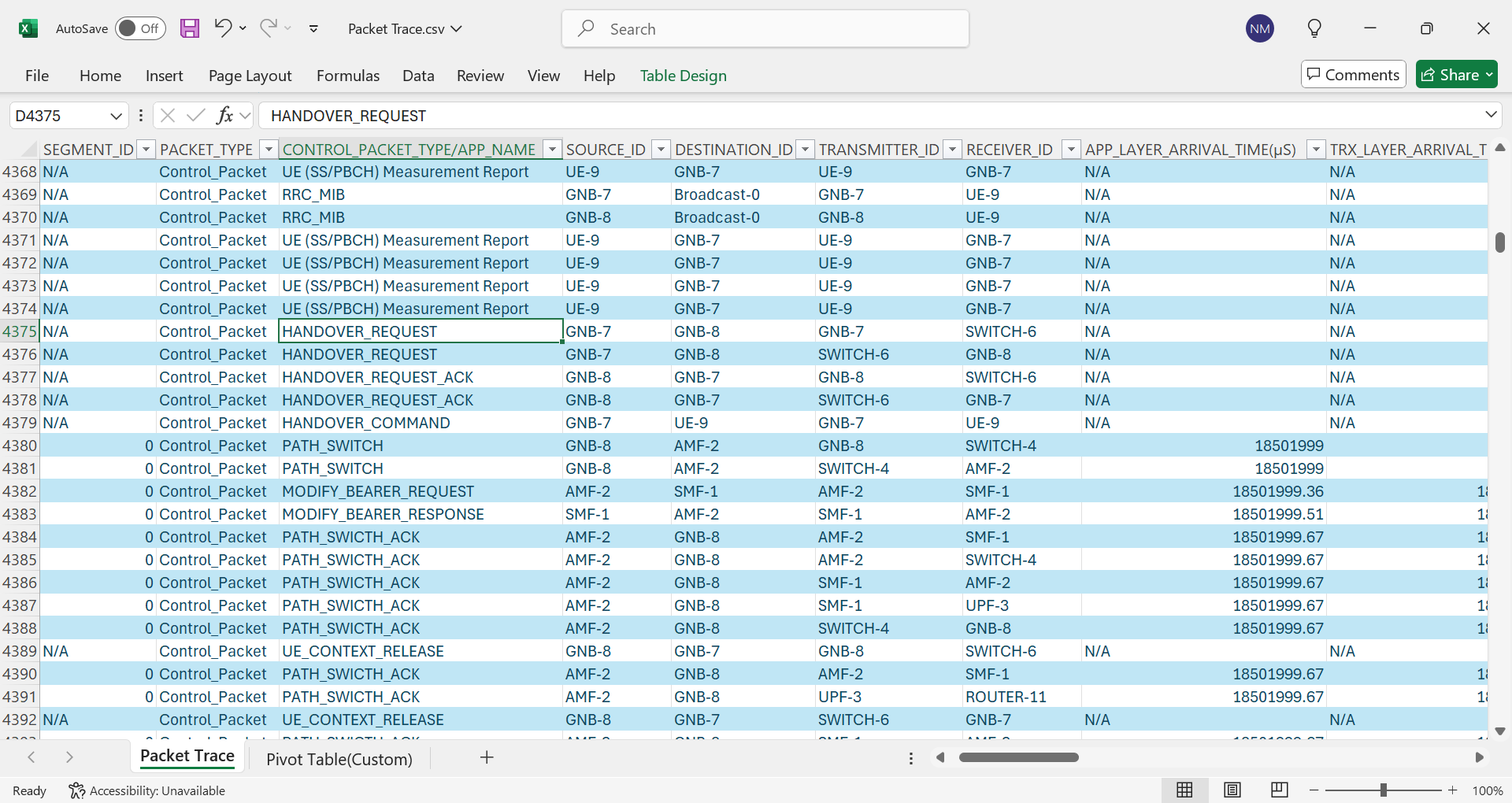
Step 8: Packet Trace is enabled by clicking on Configure reports tab. At the end of the simulation, a very large .csv file contains all the packet information and is available for the users to perform packet level analysis.
Step 9: LTENR Radio measurement, Handover log and SNR vs Time plot under LTENR Radio Measurements plots are enabled by clicking on plots/logs from right panel for detailed analysis.
Step 10: Run the Simulation for 50 Seconds.
Results and Discussion
Handover Signaling

The packet flow depicted above can be observed from the packet trace.
UE will send the UE MEASUREMENT REPORT every 5 ms to the connected gNB
The initial UE-gNB connection and UE association with the core takes place by transferring the RRC and Registration, session request response packets.
As Per the configured file-based mobility, UE 9 moves towards gNB 8.
After 18.5 s gNB 7 sends the HANDOVER REQUEST to gNB 8.
gNB 8 sends back HANDOVER REQUEST ACK to gNB 7.
After receiving HANDOVER REQUEST ACK from gNB 8, gNB 7 sends the HANDOVER COMMAND to UE 9
After the HANDOVER COMMAND packet is transferred to the UE, the target gNB will send the PATH SWITCH packet to the AMF via Switch 4.
When the AMF receives the PATH SWITCH packet, it sends MODIFY BEARER REQUEST to the SMF
The SMF on receiving the MODIFY BEARER REQUEST provides an acknowledgement to the AMF.
On receiving the MODIFY BEARER RESPONSE from the SMF, AMF acknowledges the Path switch request sent by the target gNB by sending the PATH SWITCH ACK packet back to the target gNB via Switch 4.
The target gNB sends CONTEXT RELEASE to source gNB, and the source gNB sends back CONTEXT RELEASE ACK to target gNB. The context release request and ack packets are sent between the source and target gNB via Switch 6.
RRC Reconfiguration will take place between target gNB and UE 9.
The UE 9 will start sending the UE (SS/PBCH) MEASUREMENT REPORT to gNB 8.
Plot of SNR vs. Time

This chart can be obtained in NetSim by enabling the option to plot SNR vs. time prior to the simulation. First, plot the SNR curve for gNB7 and UE9 keeping the channel as SSB. Then select “Add as new series” and select the gNB/eNB as gNB8 and UE name as UE9. Click on plot, and you would then obtain the above “stacked” plot
At 15.6 seconds, the signal-to-noise ratio (SNR) from both gNB7 and gNB8 is 16.84 dB. This is the point where the SNR curves for both gNBs intersect.
At 18.6 seconds, the SNR from gNB7 is 15.21 dB and the SNR from gNB8 is 18.54 dB. This is the point where Adj cell RSRP from gNB8 exceeds the serving cell RSRP by the handover margin (HOM) of 3 dB.
Throughput and delay variation during handover
NetSim UI displays the configuration file corresponding to this experiment as shown below.

Procedure for Effect of Handover on Delay and Throughput
The following set of procedures were done to generate this sample:
Step 1: A network scenario is designed in NetSim GUI consisting of 2 gNBs, 5G Core, 1 Router, 1 Wired Node and 1 UE in the “5G NR” Network Library.
Step 2: The device positions are set as per the table given below.
| gNB 7 | gNB 8 | UE 9 | |
|---|---|---|---|
| X Coordinate | 500 | 4500 | 500 |
| Y Coordinate | 500 | 500 | 1000 |
Sep 3: Click on the gNB 7 and expand the right-hand side properties, and set as following
| Interface (5G RAN) Properties | Value |
|---|---|
| CA Type | Single Band |
| CA Configuration | n78 |
| CA Count | 1 |
| Component Carrier 1 | Component Carrier 1 |
| DL UL Ratio | 4:1 |
| Numerology | 0 |
| Channel Bandwidth (MHz) | 10 |
| PRB Count | 52 |
| PDSCH Configuration | |
| MCS Table | QAM64 |
| X Overhead | XOH0 |
| PUSCH Configuration | |
| MCS Table | QAM64 |
| CSI Report Configuration | |
| CQI Table | Table 1 |
| Channel Model | |
| Pathloss Model | 3GPP TR 38.901-7.4.1 |
| Outdoor Scenario | Urban Macro |
| LOS_NLOS Selection | User Defined |
| LOS Probability | 1 |
| Shadow Fading Model | None |
| Fast Fading Model | No Fading |
| Additional Loss Model | None |
Similarly, it is set for gNB 8.
Step 4: The Tx Antenna Count was set to 2 and Rx Antenna Count was set to 1 in gNB \(>\) Interface (5G RAN) \(>\) Physical Layer.
Step 5: The Tx Antenna Count was set to 1 and Rx Antenna Count was set to 2 in UE \(>\) Interface (5G RAN) \(>\) Physical Layer.
Step 6: In the position properties of UE 9, set Mobility Model as File Based Mobility.
Step 7: The BER and propagation delay was set to zero in all the wired links.
Step 8: Configure application between server and UE by selecting an application from Set Traffic Tab. Click on the application flow App1 CBR, expand the application property panel on the right and set the start time to 1 s, QOS to UGS and Inter arrival time to 233.6 \(\mu\)s by keeping the packet size as default.
Additionally, the “Start Time(s)” parameter is set to 1, while configuring the application.
File Based Mobility:
In File Based Mobility, users can write their own custom mobility models and define the movement of the mobile users. Create a mobility.csv file for UE’s involved in mobility with each step equal to 0.5 sec with distance 50 m.
The NetSim Mobility File (mobility.csv) format is as follows:
| #Time(s) | Device ID | X | Y | Z |
|---|---|---|---|---|
| 0 | 9 | 500 | 1000 | 0 |
| 0.5 | 9 | 750 | 1250 | 0 |
| 1 | 9 | 1000 | 1500 | 0 |
| 1.5 | 9 | 1250 | 1750 | 0 |
| 2 | 9 | 1500 | 2000 | 0 |
| 2.5 | 9 | 1750 | 2250 | 0 |
| 3 | 9 | 2000 | 2500 | 0 |
| 3.5 | 9 | 2250 | 2750 | 0 |
| 4 | 9 | 2500 | 3000 | 0 |
| 4.5 | 9 | 2750 | 2750 | 0 |
| 5 | 9 | 3250 | 2250 | 0 |
| 5.5 | 9 | 3500 | 2000 | 0 |
| 6 | 9 | 3750 | 1750 | 0 |
| 6.5 | 9 | 4000 | 1500 | 0 |
| 7 | 9 | 4250 | 1250 | 0 |
| 7.5 | 9 | 4500 | 500 | 0 |
Step 9: The LTENR Radio measurement log file can be enabled per the information provided in Section 3.20 of 5G technology library document and enable the Latency vs. Time and Throughput vs. Time under application performance plots
Step 10: Run the Simulation for 20 Seconds.
Results and Discussion
UDP Throughput Plot
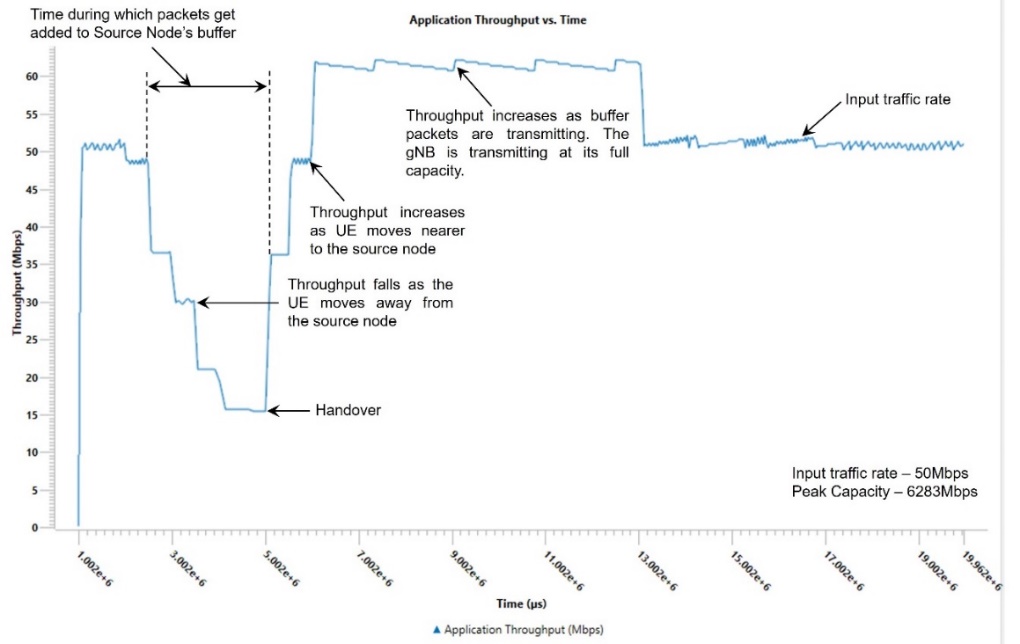
The application starts at 1 s. The generation rate is 50 Mbps and we see the network is able to handle this load, and the throughput is equal to the generation rate. We then observe that the throughput starts dropping from 2.5 s onwards because the UE is moving away from the gNB. As it moves as the SNR falls, and therefore a lower MCS is chosen leading to reduced throughput. At 3 s there is a further drop in throughput and then a final dip at 3.9 s. The time the handover occurs is 5.04 sec. At this point we see the throughput starts increasing once UE attaches to gNB8. The throughput for a short period of time is greater than 50 Mbps because of the transmission of queued packets in the s-gNB buffer which get transferred to the t-gNB buffer over the Xn interface.
UDP Delay Plot

Since the application starts at 1 s, the UDP plot begins at 1000 ms. The initial UDP delay is \(\approx 1\) ms, and hence the curve is seen as close to 0 on the Y axis. We then see that the packet delay starts increasing as the UE moves away from the gNB. This is because the link capacity drops as the CQI falls. The peak delay experienced shoots up to \(\approx\)1.1 s at \(\approx\)5.5 s when the handover occurs. Once the handover is complete the delay starts reducing and returns to \(\approx 1\) ms. The reason is that as the UE moves closer to the gNB its CQI increases and hence the 5G link can transmit at a higher rate.
Impact of Handover margin and Time-To-Trigger on the performance of a 5G heterogeneous network
In a 5G heterogeneous network we analyze how the handover margin and time-to-trigger parameters influence two performance metrics: the number of handovers and the sum throughput (aggregate throughput of all UEs).
Open NetSim, Select Examples \(\rightarrow\) 5G NR \(\rightarrow\) Impact of Handover margin and Time-To-Trigger on the performance of a 5G heterogeneous network, then click on the tile in the middle panel to load the example as shown in below screenshot.

The following network diagram illustrates what the NetSim UI displays while opening the example configuration file.

System model
The study is based on a 3-tier 5G HetNet simulation. The network comprises gNB tiers at 1.5 GHz, 2.1 GHz, and 3.5 GHz.
Each tier has a specific pathloss exponent influencing signal attenuation. The transmit power, antenna types (sector and omni-directional), and antenna heights vary across tiers. The simulation area is 10 km\(^2\), with 60 User equipments (UEs) distributed randomly and 18 tier-I gNBs, 18 tier-II gNBs, and 12 tier-III gNBs distributed randomly. The gNBs across tiers will not interference since they operate at different frequencies.
Simulation parameters include gNB and UE antenna configurations, pathloss models, interference models, and mobility settings. Shadowing effects are modeled using a lognormal distribution with a standard deviation of 5 dB.
| Parameter | Value |
|---|---|
| Simulation Area | 10 km \(\times\) 10 km |
| Number of UEs | 60 (distributed randomly) |
| Number of Tier 1 gNBs | 18 (distributed randomly) |
| Number of Tier 2 gNBs | 18 (distributed randomly) |
| Number of Tier 3 gNBs | 12 (distributed randomly) |
| gNB Tx\(\times\)Rx Antenna Count | 1\(\times\)1 |
| UE Tx\(\times\)Rx Antenna Count | 1\(\times\)1 |
| gNB Pathloss Model | Log Distance |
| Downlink Interference Model | Exact Geometric Model |
| Mobility Model | Random Walk |
| Velocity | 33 m/s |
| Calculation (update) interval for mobility | 0.12 s (120 ms) |
| Measurement Interval (ms) | 160 |
| Shadowing | Lognormal. Std. dev. = 5 dB |
| Time to trigger (ms) | Varies; 128, 256, 512, 1024 |
| Handover Margin (dB) | Varies; 0, 1, 2, 3, 4, 5, 6 |
| Handover model | A3 event based |
| Simulation Time | 30 s |
| Traffic model | Saturated (full buffer) DL |
The Time to Trigger (TTT) and Handover Margin (HO Margin) are variables in the study. An A3 event-based handover model is used. An Event A3-based HO is triggered when,
The SINR of a user from target gNB becomes higher than the SINR of the user from the serving gNB by an offset. This offset is termed as handover margin.
And this condition (C1) is maintained for a duration known as the time to trigger.
The model focuses on the interaction of these parameters and their effect on network performance, measured in terms of handover count and sum throughput.
Procedure to simulate the scenario using Multiparameter Sweeper
Click on the first experiment tile to open the scenario in NetSim. Save this scenario and open the experiment in the file explorer and open Configuration.netsim in Visual Studios.

Within the Datalink Layer of all gNB, in HANDOVER tag replace the HANDOVER_MARGIN=“{1}” and TIME_TO_TRIGGER=“{0}” representing an input variable for the multi-parameter sweeper.

Save the configuration file and rename it as input.xml.
Download the multi-parameter sweeper from the link https://github.com/NetSim-TETCOS/5g-Heterogeneous-Networkv14.4/archive/refs/heads/main.zip
Paste input.xml and Config support folder into the 5g-Heterogeneous-Networkv14.3 folder.
Open the multi-parameter-sweeper.py file in text editor, change the NETSIM_PATH suitably (line #14).

Run via CLI from 5g-Heterogeneous-Networkv14.3 folder as shown below.

The multi-parameter sweeper runs a total of 28 simulations, varying handover margin from 0 to 6 dB and time to trigger from 128, 256, 512, 1024 for all gNB’s. It generates an output file named “result.csv” which stores sum throughputs of all applications and the handover count. (It took us approximately 4 hours to complete all 28 simulations; we used a machine with a i5 processor and with 8 GB RAM).
Results and discussion
We tabulate below the handover count and sum throughput for various values of time to trigger (ms) and Handover margin (dB) which is obtained in results.csv file in multiparameter sweeper folder.
| Time-to-trigger (ms) | Handover margin (dB) | Sum throughput (Mbps) | Handover count |
|---|---|---|---|
| 128 | 0 | 215.79 | 388 |
| 128 | 1 | 225.67 | 398 |
| 128 | 2 | 213.57 | 417 |
| 128 | 3 | 203.35 | 296 |
| 128 | 4 | 219.49 | 254 |
| 128 | 5 | 212.31 | 197 |
| 128 | 6 | 215.51 | 213 |
| 256 | 0 | 215.13 | 226 |
| 256 | 1 | 205.74 | 199 |
| 256 | 2 | 212.15 | 164 |
| 256 | 3 | 207.26 | 140 |
| 256 | 4 | 210.16 | 101 |
| 256 | 5 | 215.91 | 94 |
| 256 | 6 | 216.96 | 86 |
| 512 | 0 | 210.15 | 67 |
| 512 | 1 | 215.89 | 76 |
| 512 | 2 | 219.47 | 44 |
| 512 | 3 | 207.39 | 38 |
| 512 | 4 | 216.99 | 31 |
| 512 | 5 | 213.75 | 21 |
| 512 | 6 | 208.79 | 20 |
| 1024 | 0 | 217.39 | 23 |
| 1024 | 1 | 204.60 | 21 |
| 1024 | 2 | 207.97 | 18 |
| 1024 | 3 | 212.28 | 14 |
| 1024 | 4 | 213.46 | 15 |
| 1024 | 5 | 200.06 | 11 |
| 1024 | 6 | 200.10 | 8 |

It is evident from the plot that the handover count decreases as the handover margin increases. This trend is consistent across different TTT values, suggesting that a higher handover margin generally results in fewer handovers. The rationale behind this trend is that increased handover margin leads to more stringent conditions for handover and thereby reduces the frequency of handover occurrences.
We also observe that the handover count decreases as TTT increases. Shorter TTT values lead to quicker responses to signal changes, resulting in more frequent handovers, while longer TTT values delay the handover process, thereby reducing the handover count. The plot highlights the effects of both the handover margin and the TTT on handover count.

In the second chart we see that sum throughput generally rises and then falls with the increasing handover margin. For each handover margin we see the throughput again roughly increases and then drops as TTT increases. Initially, with a higher handover margin and/or higher TTT unnecessary and frequent handovers between cells are avoided. This leads to better throughput, but only to a certain extent. Beyond a point, a high handover margin and/or high TTT causes delayed handovers. Users stay connected to a weaker cell longer, despite being closer to a stronger cell, leading to poorer signal quality and thus lowering throughput.
QoS in 5G using GBR
Introduction
This experiment explores a new approach to providing Quality of Service (QoS) guarantees in 5G networks by modifying the traditional Proportional Fair Scheduling (PFS) algorithm. The study focuses on implementing Guaranteed Bit Rate (GBR) requirements using index bias (Lagrange multiplier) in the scheduler, and understanding how this modification impacts network performance under various scenarios.
The experiment investigates three cases: First, a baseline scenario using standard PFS where all User Equipment (UEs) are static but at different distances from the gNB (base station). Second, the same setup but with the modified PFS algorithm incorporating GBR guarantees for one UE. Finally, the study examines how the GBR mechanism performs when one UE is mobile. In all cases, we simulate Rayleigh fading channels between the gNB and UEs, creating dynamic channel conditions that reflect real-world wireless propagation.
Through these scenarios, the experiment demonstrates how the scheduler dynamically adjusts resource allocation to maintain throughput guarantees for specific UEs, at the expense of reducing resources to other users. The study is particularly useful for understanding how modern 5G networks can provide differentiated services and maintain quality guarantees in real-world conditions, where users may be at varying distances from the base station and potentially mobile.
Methodology
Open NetSim and click on Examples \(>\) 5G NR \(>\) QoS in 5G using GBR then click on the tile in the middle panel to load the example as shown below

Case 1: Proportional Fair Scheduling (PFS). All UEs are static
NetSim UI displays the configuration file corresponding to this experiment as shown below

Set grid length as 6000 m and width as 12000 m from grid property panel on the right.
Set distance as follows:
gNB 9 to UE 10 = 1500 m
gNB 9 to UE 11 = 2000 m, and
gNB 9 to UE 12 = 2500 m
Go to gNB properties \(\rightarrow\) Interface (5G RAN), set the following properties as shown below Table. In the first case the scheduling type is set to PFS.
| Properties | Value |
|---|---|
| Datalink Layer Properties | |
| Scheduling Type | PFS, PFS with RG |
| Physical Layer Properties | |
| CA Type | Single band |
| CA Configuration | n78 |
| CA1 | |
| Numerology | 1 |
| Channel Bandwidth | 100 MHz |
| Channel Model | |
| Pathloss Model | 3GPP TR 38.901-7.4.1 |
| Outdoor Scenario | Urban Macro |
| LOS NLOS Selection | User defined |
| LOS Probability | 1 |
| Shadow Fading Model | None |
| Fast Fading Model | No fading |
Set Tx Antenna Count as 1 and Rx Antenna Count as 1 in gNB properties.
Set Tx Antenna Count as 1 and Rx Antenna Count as 1 in all the UEs.
Go to the Set Traffic tab in the top ribbon and create a CBR application as shown in the table below. To change the transport protocol, QoS, and IAT click on the application and change the properties in the right-side property panel.
| Application Properties | Application 1 | Application 2 | Application 3 |
|---|---|---|---|
| Application Type | CBR | CBR | CBR |
| Source ID | 8 | 8 | 8 |
| Destination ID | 10 | 11 | 12 |
| QoS | UGS | UGS | UGS |
| Transport Protocol | UDP | UDP | UDP |
| Packet Size | 1460 Bytes | 1460 Bytes | 1460 Bytes |
| Inter-arrival time | 58.4 \(\mu\)s | 58.4 \(\mu\)s | 58.4 \(\mu\)s |
| Start Time | 1 s | 1 s | 1 s |
Make sure you enable these two plots under plots section as shown in figure

Run Simulation for 100 s and note down throughput value in the results window for each UE.
Here, we can see the resulting plots of the case:

Case 2: PFS with RG using Guaranteed Bit Rate (GBR). All UEs are static.
Now, for the same scenario above we just need to disable the GBR Configuration.
For doing that we need to change the Scheduling algorithm from Proportional Fair to PFS with RG as shown below.

Then, Configure GBR UEs via GUI as shown below. Change the Downlink of UE12 to 27.57 Mbps and click on update.

Now, run the scenario for 100 s.
Now plot the values using plots section in Results dashboard.


Case 3: PFS with RG using GBR. One of the UE’s is mobile.
In this case we are working with GBR again.
Now we need to add Mobility for UE-12, click on UE-12 then select Position \(\rightarrow\) Mobility Model \(\rightarrow\) File Based Mobility \(\rightarrow\) via File.

Now add Mobility as shown below:
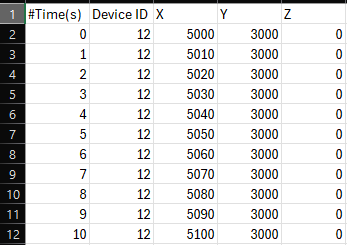
In this way, you can add mobility by increasing 10 m of distance in the interval of 1 s and keep adding up to 100 s then save the file.
Now, run the simulation for 100 s.
The plots are obtained from results dashboard:
So, we can see a lot of spike variations in plots due to mobility in UE 3.


Obtaining the EWMA MAC Throughput and Resource share
Now, let’s see the MAC Throughputs, to obtain them follow the steps:
Select the Logs section in Result Metrics, then click on LTENR Radio Resource Allocation.csv log file as shown below.

After the log file is loaded into the excel sheet, select on the pivot table section below and select the checkboxes of UE ID and EWMA MAC throughput on the right side.
Now drag the UE ID to the rows and EWMA MAC throughput to the values of the table and change the values from sum to average by right clicking on that column head as shown below.

Now in the sheet table, you can see the MAC Throughput values of respective UEs to the right side of them under the ‘Total’ named column.
In this way, you can obtain the MAC Throughput values of 3 UEs in all the three cases using the LTENR Radio Resource Allocation.csv log file.
The values obtained from all the cases are tabulated in Results.
Now, to obtain Allocated PRBs percentage:
Follow step 1, and then instead of adding EWMA MAC Throughput add Allocated PRBs to Values section.
Now, right click on the values and select ‘show values as’ section then select ‘% of Grand Total’ and click on OK as shown below.

On the left side table, you can see the values.
The values obtained from all the cases are tabulated in Results.
Results and Discussion
Let’s analyze the Application Throughputs and MAC Throughputs obtained by 3 UEs in results dashboards in all the three different cases discussed above:
| Case # | Description | UE1 (Mbps) | UE2 (Mbps) | UE3 (Mbps) |
|---|---|---|---|---|
| 1 | Proportional Fair Scheduling (PFS). All UEs static. | 64.65 | 37.22 | 19.59 |
| 2 | PFS with RG using Guaranteed Bit Rate (GBR). All UEs static. | 61.26 | 35.27 | 21.64 |
| 3 | PFS with RG using GBR. UE 3 is mobile. | 33.23 | 19.13 | 20.83 |
| Case # | Description | UE1 (Mbps) | UE2 (Mbps) | UE3 (Mbps) |
|---|---|---|---|---|
| 1 | Proportional Fair Scheduling (PFS). All UEs static. | 82.34 | 47.40 | 24.59 |
| 2 | PFS with RG using GBR. All UEs static. | 78.03 | 44.92 | 27.56 |
| 3 | PFS with RG using GBR. UE 3 is mobile. | 42.34 | 24.38 | 26.53 |
| Case # | Description | UE1 (%) | UE2 (%) | UE3 (%) |
|---|---|---|---|---|
| 1 | Proportional Fair Scheduling (PFS). All UEs static. | 33.33 | 33.33 | 33.33 |
| 2 | PFS with RG using GBR. All UEs static. | 31.59 | 31.59 | 36.83 |
| 3 | PFS with RG using GBR. UE 3 is mobile. | 17.14 | 17.14 | 65.73 |
Case-1: Proportional Fair (PF) Algorithm
Under standard PFS, the algorithm distributes Physical Resource Blocks (PRBs) uniformly among the three UEs, with each receiving approximately 33.33% of the resources. This results in decreasing throughputs as distance from the gNB increases – UE1 achieves 64.65 Mbps, UE2 gets 37.22 Mbps, and UE3 receives 19.59 Mbps at the application layer.
Case-2: GBR with Static UEs
When GBR is enabled for UE3 with a target rate of 27.57 Mbps, we observe the index bias mechanism actively working to guarantee this rate. The scheduler increases the bias factor for UE3, resulting in its PRB allocation increasing from 33.33% to 36.83%.
This resource reallocation successfully raises UE3’s throughput from 19.59 Mbps to 21.64 Mbps at the application layer, achieving the target MAC layer throughput of 27.56 Mbps.
However, this comes at the cost of reduced resources for other UEs – UE1’s throughput drops from 64.65 Mbps to 61.26 Mbps, and UE2’s decreases from 37.22 Mbps to 35.27 Mbps.
Case-3: GBR with Mobile UE
As UE3 begins moving away from the gNB, we observe a complex interplay between distance, channel conditions, and the index bias mechanism.
Initially, as UE3’s throughput starts dropping due to increased distance, the index bias increases to compensate, pulling more resources from UE1 and UE2. Their throughputs drop significantly – UE1 falls to 33.23 Mbps and UE2 to 19.13 Mbps.
As UE3 moves even further away, the scheduler dramatically increases the index bias in an attempt to maintain the GBR. This results in UE3 being allocated nearly 65.73% of all PRBs, leaving only about 17.14% each for UE1 and UE2.
Despite this extreme resource reallocation, UE3’s throughput still falls to 20.83 Mbps, unable to meet the GBR target due to poor channel conditions at the increased distance. Meanwhile, the throughputs of UE1 and UE2 are severely impacted due to their minimal resource allocation.
This behavior demonstrates both the power and limitations of the index bias mechanism in GBR implementation – while it can effectively guarantee bit rates under most conditions by redistributing resources, there are physical limitations that cannot be overcome simply by increasing resource allocation when channel conditions become too poor.